
We consider two interacting qubits connected through a harmonic oscillator to an Ohmic bath16 (see Fig. 1a). In a related study29, we explored the effects of changing the spectral density of the bath from Ohmic to sub-Ohmic and super-Ohmic. We set ℏ = kB = 1 and the Hamiltonian that describes the system is given by: H = HS + HB + HS−B. Here, the system (qubits and oscillator) energy HS is defined as:
$${H}_{S}=-\frac{\Delta }{2}\left({\sigma }_{x}^{1}+{\sigma }_{x}^{2}\right)+\frac{J}{4}{\sigma }_{z}^{1}{\sigma }_{z}^{2}+{\omega }_{0}{a}^{{\dagger} }a+g(a+{a}^{{\dagger} })\left({\sigma }_{z}^{1}+{\sigma }_{z}^{2}\right),$$
(1)
where Δ is the frequency of the two qubits, J is the strength of the interaction between them, and \({\sigma }_{i}^{j}\) (with i = x, y, z and j = 1, 2) are the Pauli matrices. The oscillator frequency is ω0, and a (a†) are the annihilation (creation) operators. The parameter g represents the coupling strength between the qubits and the oscillator. We emphasize that there should be a self-interaction, dipole-dipole term between the qubits which ensures an exact cancellation at zero frequency with the cavity-mediated interaction, as expected from gauge invariance30. This term is proportional to \({S}_{z}^{2}=({\sigma }_{z}^{1}+{\sigma }_{z}^{2})/4\). By expanding this square, we obtain two terms proportional to the identity operator on the two-qubit system, and the last term takes the form \(\frac{{g}^{2}}{2{\omega }_{0}}{\sigma }_{z}^{1}{\sigma }_{z}^{2}\). This can be interpreted as an additional interaction between the two qubits due to the presence of the cavity. In this context, our J in Equation (1) represents an effective interaction that also accounts for this additional term.
The bath Hamiltonian and its interaction with the system are given by:
$${H}_{B}+{H}_{S-B}={\sum }_{i=1}^{N}\left[\frac{{p}_{i}^{2}}{2{M}_{i}}+\frac{{k}_{i}}{2}{({x}_{0}-{x}_{i})}^{2}\right].$$
(2)
The bath is represented as a collection of N oscillators with frequencies \({\omega }_{i}=\sqrt{\frac{{k}_{i}}{{M}_{i}}}\), and coordinates and momenta are denoted by xi and pi, respectively. Additionally, x0 denotes the position operator of the resonator with mass m: \({x}_{0}=\sqrt{\frac{1}{2m{\omega }_{0}}}(a+{a}^{{\dagger} })\). This interaction with the bath describes dissipation as proposed by Caldeira-Leggett31,32. The key challenge for implementing our model is to reach our regime of very strong coupling. There are experimental platforms where this parameter regime can be obtained33. One relevant possibility is a flux qubit ultrastrongly coupled to a dissipative resonator34,35,36,37. This system is useful for describing the regime beyond strong coupling. A dissipative resonator can be conceptualized as an oscillator coupled to a bath, imparting a finite decay time and other effects if the coupling is strong. Hence, in our model, we connect the oscillator to an Ohmic bath. In5, we proposed realizing this model by adding a series of resistors to a flux qubit interacting with its resonator in Figures 6 and 7 of Supplemental Material.
The coupling to the bath induces renormalization effects on several parameters: the oscillator frequency \({\bar{\omega }}_{0}\), as well as the interaction strengths ḡ and \(\bar{{g}_{i}}\) (further detailed in Methods Sec. Time-dependent variational principle numerical simulations). This results in the following bath spectral density \(J(\omega )={\sum }_{i = 1}^{N}\frac{{k}_{i}{\omega }_{i}}{4m{\bar{\omega }}_{0}}\delta (\omega -{\omega }_{i})=\frac{\alpha }{2}\omega f\left(\frac{\omega }{{\omega }_{c}}\right)\) where α controls the system-bath coupling. Here \(f\left(\frac{\omega }{{\omega }_{c}}\right)\) is a function that depends on the cutoff frequency for the bath modes, ωc, which governs the behavior of the spectral density at high frequencies. This function is taken as \(f\left(\frac{\omega }{{\omega }_{c}}\right)=\Theta \left(\frac{{\omega }_{c}}{\omega }-1\right)\), where Θ(x) is the Heaviside step function. The cutoff frequency is typically chosen to be the largest energy scale in the system. In the following we set: ω0 = Δ, J = − 10Δ (ferromagnetic interaction) and J = 0 (antiferromagnetic interaction), α = 0.1, ωc = 30Δ.
It is worth noticing that the system can be mapped to an equivalent model of two interacting qubits in contact, through σz, with a structured bath whose spectral density shows a peak at the oscillator frequency5,38 (see Equation (5)). The spectrum of the two-qubit Hamiltonian, Hqub = HS(g = 0), is shown in Fig. 1b.
QPT evidences at thermodynamic equilibrium
We first investigate the equilibrium properties of the system, using two different approaches. The first method is the WLMC approach, which is based on path integrals5,29,39 (see Methods Sec. Worldline Monte Carlo method). Here, the structured bath degrees of freedom are eliminated, resulting in an effective Euclidean action5,32,40,41, with the kernel expressed in terms of the structured spectral density J(ω). This structure is characteristic of a spin-boson model but is now extended to involve two qubits interacting with the bath, as outlined in34,38 (see Methods Sec. Time-dependent variational principle numerical simulations). This transformation leads to a classical system of spin variables distributed along two chains, each of them with length β = 1/T. The spins experience long-range ferromagnetic interactions both within each chain and between the two chains. The functional integral is computed using a Poissonian measure and adopts a hybrid algorithm40,42, based on an alternation of Wolff’s43 and Metropolis moves. We find that, as ω0 remains constant and β tends toward infinity, the kernel displays a power asymptotic behavior, K(τ) ≃ 1/τ2. This power-law behavior with an exponent of 2 determines the onset of a Beretzinski-Kosterlitz-Thouless (BKT) QPT. In the Supplementary Note 1 we perform a BKT scaling for a parameter regime that allows for feasible numerical analysis and confirm that the nature of the transitions is indeed BKT (see Supplementary Fig. 1) for the other parameter regimes analyzed in the paper, as they belong to the same universality class. In this respect, another interesting experimental challenge could be the possibility of observing the interplay between short-range and long-range interactions in relation to DQPTs.
The second method we employ is the DMRG (see Methods Sec. Density-matrix renormalization group algorithm), an adaptive algorithm for computing eigenstates of many-body Hamiltonians. It is particularly effective for calculating low-energy properties of one-dimensional and two-dimensional quantum systems. DMRG uses the MPS representation to determine the ground state of low-dimensional quantum systems. In particular, we use the ITensor library44 for a system with a bath of N = 300 harmonic oscillators.
Squared magnetization, interaction energy, and entanglement
In Fig. 2a, we present the squared magnetization of the qubits, defined as \({M}^{2}=\frac{1}{4\beta }\int_{0}^{\beta }d\tau \langle ({\sigma }_{z}^{1}+{\sigma }_{z}^{2})(\tau )({\sigma }_{z}^{1}+{\sigma }_{z}^{2})(0)\rangle\), where τ labels the positions of the spins on the two equivalent chains (corresponding to the two spins labeled by the superscripts 1 and 2), after eliminating the bath degrees of freedom in favour of an effective classical system of spins as discussed in ref. 34 (see Methods Sec. Worldline Monte Carlo method). We plot this magnetization as a function of g/Δ for three different inverse temperatures, βΔ = {100, 500, 1000}. The data obtained using WLMC method exhibit a crossover for M2 from 0 to 1 increasing g/Δ that becomes sharper and sharper lowering the temperature. This behavior suggests the occurrence of the BKT QPT, which is estimated to set in at a critical value of gc ≈ 0.5Δ from βΔ = 103 data. Additionally, we calculate the mean value of the interaction Hamiltonian between the two qubits, denoted as \(\langle {H}_{J}\rangle =J\langle {\sigma }_{z}^{1}{\sigma }_{z}^{2}\rangle /4\), as a function of g/Δ for the same three temperature values (see Fig. 2b). We emphasize that both the WLMC and DMRG methods yield consistent results. Note that the interaction becomes more negative with increasing values of g since the bath induces an effective ferromagnetic coupling between the spins.
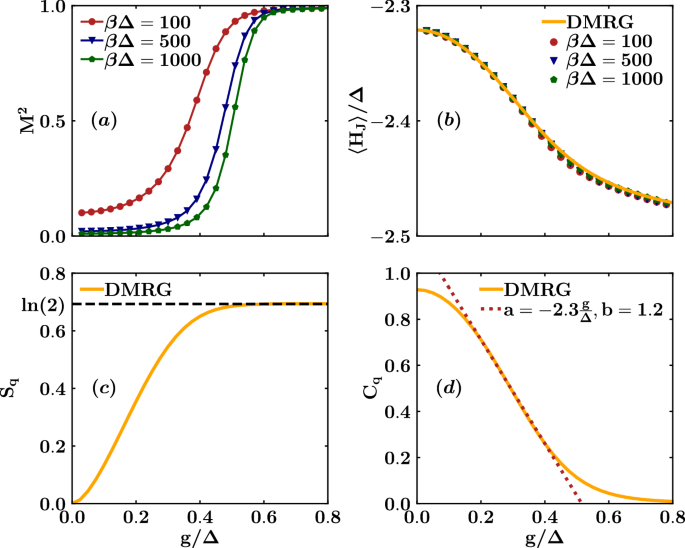
Qubits’ squared magnetization M2 (a), interaction energy between the qubits 〈HJ〉/Δ (b), von Neumann entropy Sq (c) and concurrence Cq (d) as functions of g/Δ for J = − 10Δ, computed through WLMC and DMRG. For the WLMC method the calculations are made for βΔ ∈ [100, 1000]. In panel (c), the dashed line represents the maximum von Neumann entropy for a single qubit. In panel (d), the dotted line indicates a linear fit of the concurrence performed near the transition, which intersects the g-axis at approximately the critical value.
To analyze the entanglement properties of the system in the presence of the QPT, we determine the qubits’ density operator ρq and compute the qubits’ entropy, denoted as \({S}_{q}=-\,{\mbox{Tr}}\,\{{\rho }_{q}\ln {\rho }_{q}\}\), and the concurrence, given by \({C}_{q}=\max (0,{\lambda }_{1}-{\lambda }_{2}-{\lambda }_{3}-{\lambda }_{4})\). Here, λi represents the eigenvalues of the Hermitian matrix \(\sqrt{\sqrt{{\rho }_{q}}\widetilde{{\rho }_{q}}\sqrt{{\rho }_{q}}}\), and \(\widetilde{{\rho }_{q}}=({\sigma }_{y}^{1}\otimes {\sigma }_{y}^{2}){\rho }_{q}^{* }({\sigma }_{y}^{1}\otimes {\sigma }_{y}^{2})\), with * indicating complex conjugation. In Fig. 2c, d, we present the entropy and entanglement as functions of g/Δ, computed using the DMRG algorithm. The entropy increases for values of g near the critical point, approaching a value of approximately \(\ln (2)\) just at the critical values determined by the WLMC approach. We also notice the similarity between Fig. 2a, c. In contrast, as shown in Fig. 2d, the concurrence decreases as a function of g, approaching zero. Moreover, through a linear fit of the concurrence within the critical region (Cq = ag/Δ + b in Fig. 2d), it becomes evident that the line intersects the g-axis at approximately g ≈ 0.5Δ, a value close to the estimated critical point. This behavior can be explained by the qubits approaching a two-degenerate state at the BKT QPT, where they are either both in the “up” or “down” state. This clearly results from a lack of entanglement between the two qubits and an enhancement of entanglement of each of them with the bath39.
Now we conduct the same analysis at thermodynamic equilibrium for the case of zero interaction J between the two qubits. Here, we demonstrate the agreement in thermodynamic quantities computed through both DMRG and WLMC methods. Figure 3a presents the squared magnetization of the qubits (M2), plotted as a function of g/Δ for two different inverse temperatures, βΔ = 100 and βΔ = 1000. With the WLMC method, we observe a crossover for the squared magnetization from 0 to 1 around a critical value of gc ≈ 0.6Δ. This jump becomes more pronounced as the temperature decreases. Furthermore, we calculate the mean value of the qubits Hamiltonian, denoted as \(\langle {H}_{\Delta }\rangle =-\Delta \langle {\sigma }_{x}^{1}+{\sigma }_{x}^{2}\rangle /2\), as a function of g/Δ for the same two temperature values (see Fig. 3b). Both the WLMC and DMRG methods yield consistent results. The qubits Hamiltonian does not exhibit a jump but becomes less negative as the bath reduces the effective qubits gap with increasing values of g.
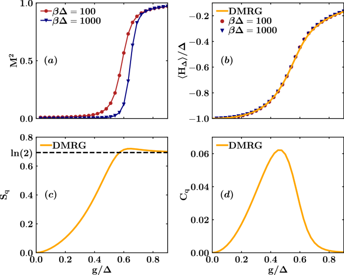
Qubits’ squared magnetization M2 (a), qubits’ energy 〈HΔ〉/Δ (b), von Neumann entropy Sq (c) and concurrence Cq (d) as functions of g/Δ for J = 0, computed through WLMC and DMRG. For the WLMC method the calculations are made for βΔ ∈ [100, 1000]. In panel (c), the dashed line represents the maximum von Neumann entropy for a single qubit.
Figure 3c, d present the entropy and entanglement as functions of g/Δ. The entropy increases for values of g near the critical point, asymptotically approaching a value of approximately \(\ln (2)\). Conversely, the concurrence is almost zero everywhere, except for a small peak near the transition. Again this behavior is consistent with the qubits approaching a two-degenerate state near the transition. The difference from the case of non-zero J is that the concurrence does not change much because the qubits prefer to entangle with the bath to facilitate the transition and entropy can be slightly greater than \(\ln (2)\).
Magnetization distribution and correlations
Since M2 displays a crossover from 0 to 1 (Fig. 2a), one naturally wonders if this is related to the onset of a BKT QPT. This question can be better addressed studying the distribution of the normalized magnetization, denoted as P(M/2). In Fig. 4, we plot the magnetization distribution for two different values of g/Δ, smaller and larger of the estimated one for BKT transition. When g = 0.21Δ gc (Fig. 4a), the distribution exhibits a single peak centered at M = 0. On the other hand, for g = 0.66Δ > gc (Fig. 4c), it acquires a bimodal character, with two peaks centered at M/2 = ±1, again with the same vanishing mean value. We emphasize that, above gc, the distribution develops two peaks that are expected to become two delta functions, centered at \(\pm \sqrt{{M}^{2}}\), in the thermodynamic limit. It’s also worth noting that the formation of a bimodal distribution is clearly related to the crossover observed in M2. This behavior, reminiscent of classical thermodynamics, signals the emergence of a QPT. In addition, we can examine the correlations \(C(\tau )=\langle ({\sigma }_{z}^{1}+{\sigma }_{z}^{2})(\tau )({\sigma }_{z}^{1}+{\sigma }_{z}^{2})(0)\rangle\) as another indicator of the occurrence of the QPT. Figure 4 shows the distinct behavior before and after the onset of the transition. Specifically, the normalized correlation function, defined as C = C(τ/(β/2))/C(0), tends toward 0 as τ approaches β/2 before the critical point (Fig. 4b) and converges to a finite value, i.e., M2, after the transition (Fig. 4d), indicating the long-range nature of the correlations between the spins above gc.
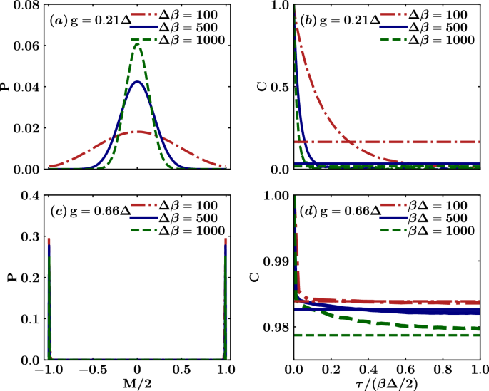
Qubits’ magnetization distribution P(M/2) ((a) and (c)) and normalized correlation function C = C(τ/(βΔ/2))/C(0) ((b) and (d)). We consider two scenarios: one with g = 0.21Δ before the transition ((a) and (b)) and another with g = 0.66Δ after the transition ((c) and (d)). These calculations are performed using the WLMC method at inverse temperatures of βΔ ∈ [100, 1000].
Dynamics of energy and entanglement
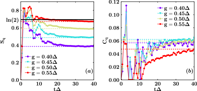
We investigate the out-of-equilibrium properties of the system, focusing on the behavior of energy and entanglement over time. To accomplish this, we employ the TDVP algorithm45,46,47 (see Methods Sec. Time-dependent variational principle numerical simulations), implemented using the ITensor library44, to evolve the wavefunction of the entire system represented as an MPS. The adoption of this technique proves advantageous for our system strongly coupled to the environment, enabling us to achieve long simulation times. Consequently, we can compare these behaviors with those computed using the DMRG at thermodynamic equilibrium. Specifically, we choose the ground state of the Hamiltonian HS(g = 0) (state \(\left\vert 0\right\rangle\) in Fig. 1) as the initial state for simulations and calculate the qubits’ von Neumann entropy Sq(t), the concurrence Cq(t), and the mean values of the various contributions to the total energy of the system, including 〈HS(t)〉, 〈HB(t)〉, and 〈HS−B(t)〉 for different values of g, crossing the critical point. Figure 5a, b demonstrate that both entropy and concurrence are approaching thermodynamic values. Moreover, the greater g, the less time the system needs to reach the equilibrium values.
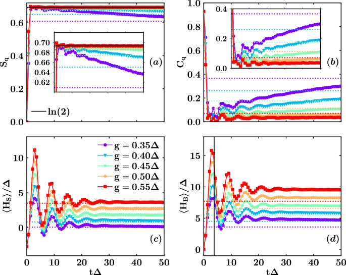
Qubits’ entropy Sq (a) and concurrence Cq (b), system energy 〈HS(t)〉/Δ (c) and bath energy 〈HB(t)〉/Δ (d) as functions of dimensionless time tΔ for different values of the coupling g ∈ [0.35, 0.55]Δ and J = − 10Δ, crossing the critical point, calculated through TDVP and DMRG. The insets in panels (a) and (b) provide a zoomed-in view of the long-time behaviors. The dotted lines represent the DMRG equilibrium values corresponding to the TDVP dynamical values, shown as solid lines with markers specified in the legend. In panel (a), the horizontal black line indicates the maximum value of von Neumann entropy for a single qubit. In panel (d), the vertical black line marks the critical time at which the DQPT occurs.
We stress that from a dynamical point of view, this model also exhibits a delocalized-localized transition. In the Rabi model, this localization physically manifests as a reduction to a sort of two-level system for the two qubits that can only be found in one of the two ferromagnetic states \(\left\vert \uparrow \right\rangle \left\vert \uparrow \right\rangle\) or \(\left\vert \downarrow \right\rangle \left\vert \downarrow \right\rangle\). While approaching the transition, there can be oscillation only between these two states, and after the transition, the qubits can only be in one of the two states. As we demonstrated in the Supplemental Material of ref. 5, one can adiabatically apply a magnetic field on the qubits or an electric field on the oscillator and examine the response function of the qubits or the oscillator, respectively. Observing the system after the critical coupling, where the equilibrium transition occurs, reveals that the system no longer relaxes and becomes localized. This is described in Supplementary Note 2 and illustrated by the oscillator relaxation function Σx in Supplementary Fig. 2, which remains constant at 1 (indicating no relaxation) after the transition. This also suggests that one can look at the oscillator, which is sensitive to the change of the quench parameter g, and it monitors the behavior of the qubits in the localization transition. Therefore, the oscillator could be useful for measuring qubits and has potential applications in quantum sensing.
The results discussed above can be understood by examining the mapped model. The effective kernel for asymptotic imaginary times (low-frequency regime) is linear in the frequency, as in the case of the Ohmic bath of a single spin-boson model. This low-frequency behavior implies an asymptotic 1/τ2 behavior that is the fingerprint of a delocalized-localized transition, observable by increasing the effective coupling. In the Rabi model, this effective coupling depends not only on the bath coupling already present in the spin-boson model but also on the coupling g and the oscillator frequency ω0.
Regarding energy contributions, as depicted in Fig. 5c, the mean value of the system’s energy 〈HS(t)〉 approaches its thermodynamic equilibrium value after approximately tΔ = 30, while the mean value of the bath energy 〈HB(t)〉 (see Fig. 5d) never reaches the DMRG values. We also computed the mean value of the interaction energy 〈HS−B(t)〉, although it is not shown here, which reaches thermodynamic equilibrium on the same time scale as the system. The total energy is conserved, the bath remains at zero temperature, but accumulating bosons, i.e., absorbing the energy difference relative to the ground-state energy calculated through DMRG. This phenomenon can also be understood in terms of quasiparticles. When the coupling g is small, the system reaches the equilibrium of its Hamiltonian HS. However, as g increases, one can envision another Hamiltonian involving non-interacting quasiparticles dressed by the bath bosons, resulting in a small residual interaction energy. Consequently, quasiparticles reach the thermodynamic equilibrium in the presence of additive free bosons that are not able to modify the bath temperature. After analyzing asymptotic times, in the following we will focus our attention on smaller time scales.
We again study the out-of-equilibrium properties in the case of J = 0, comparing long-times dynamics with thermodynamic equilibrium. Specifically, we calculate the qubits’ entropy Sq(t), and the concurrence Cq(t) for different values of g, approaching the critical point. In Fig. 6a, b, we can see that both entropy and entanglement approach their thermodynamic values at earlier times than in the J ≠ 0 case. To quantitatively understand the approach to equilibrium for these quantities, we also fitted the curves for the two values of J. This confirmed that the decay of the entropy and the saturation of the concurrence have already reached the long times necessary to observe equilibrium observables for J = 0. In contrast, for J ≠ 0, we need a time on the order of tΔ ≈ 103, which is too difficult to achieve numerically. Moreover, the greater the value of g, the more time the system needs to reach equilibrium values. This very long-time equilibration can be explained physically by noting that when J = 0, the system is directly connected to the bath, making it easier to reach thermodynamic equilibrium. In contrast, in the case of J = −10Δ, the very strong qubit-qubit interaction complicates the interplay between the internal dynamics and the equilibration process, leading to thermodynamic equilibrium being reached over much longer times.
Qubits’ entropy Sq (a) and concurrence Cq (b) as functions of dimensionless time tΔ for different values of the coupling g ∈ [0.40, 0.55]Δ and J = 0, near the critical point, computed through TDVP and DMRG. The dotted lines represent the DMRG equilibrium values corresponding to the TDVP dynamical values, shown as solid lines with markers specified in the legend. In panel (a), the horizontal black line indicates the maximum value of von Neumann entropy for a single qubit.
We do not show the time behavior of the energy contributions, but we have analyzed them, finding results similar to the interacting case. That is, the system’s energy and the interaction with the bath approach equilibrium values, while the bath’s energy remains different, accounting for the overall difference in energy due to the initial excited state.
Dynamical quantum phase transitions: Loschmidt echo
It has been demonstrated in refs. 7,8 that a closed quantum many-body system can undergo a DQPT without any external control parameters, such as temperature or pressure. The typical non-analyticities of phase transitions manifest over time in the matrix element of the system unitary evolution operator on the initial state, i.e., the Loschmidt echo \({{\mathcal{L}}}(t)\) (see Fig. 7a). To observe such a phase transition, the procedure involves preparing the system in a well determined initial state inducing a quench in a parameter on which the Hamiltonian depends. Subsequently, the system evolves with the full Hamiltonian after the quench, and the Loschmidt echo is computed over time48. It can be expressed as \({{\mathcal{L}}}(t)={e}^{-N\lambda (t)}\) taking into account the exponential dependence on the system’s degrees of freedom, denoted by N. Therefore, the rate function λ(t) (see Fig. 7b) is the key property to monitor over time in order to observe non-analyticities. Formally, there exists an equivalence between the rate function and the free energy derived from a complex partition function, demonstrating the presence of singular points. Here, we aim to compute the same quantities in the closed system, which includes the bath. We underline that we operate with the entire system energy fixed in an excited state7, whereas the QPT is studied using WLMC and DMRG, which examine the entire system’s ground state. Consequently, the dynamical behavior we observe is due to energy fluctuations above the ground state; therefore, we cannot expect the two transitions to occur at exactly the same parameter values.
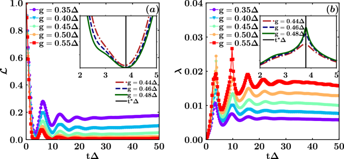
Loschmidt echo \({{\mathcal{L}}}(t)\) (a) and rate function λ(t) (b) as functions of dimensionless time tΔ for different values of the coupling g ∈ [0.35, 0.55]Δ and J = − 10Δ, crossing the critical point, computed through TDVP. The insets provide a zoomed-in view near the transition, allowing identifying the critical time t*Δ ≈ 3.8.
Figure 7 illustrates the echo and the rate function over time for different values of g around the transition. Additionally, the inset clearly demonstrates how the scalar product between the evolved state and the initial one becomes zero (see inset of Fig. 7a) and the kink becomes narrower and higher as the critical point is approached at time t*Δ ≈ 3.8 (see inset of Fig. 7b). In Fig. 5d we can see that the first maximum at short times occurs at around the critical time indicated by the black vertical line, as another marker of the transition in the dynamics. Beyond the critical region, the peak occurs at earlier times, and multiple peaks emerge over time in the rate function. This behavior occurs because the system can transition to the other phase more rapidly with higher couplings to the bath. The scalar product which vanishes indicates that the bath, including a lot of excited bosons, significantly differs from the initial vacuum state, leading to the orthogonality catastrophe, a characteristic feature of a phase transition. We emphasize that, through the quench, we are probing the first excited states and fluctuations are responsible for the observation of the DQPTs, reminiscent of the QPT occurring at thermodynamic equilibrium at zero temperature in the ground state of the entire Hamiltonian. In the Supplementary Note 3, we demonstrate that the two-qubit subsystem does not transition by computing the fidelity between the evolved state and the initial one. This fidelity coincides with the open systems generalization described in11, given that our initial state is pure. As shown in Supplementary Fig. 3, it does not vanish over time and hence its logarithm does not exhibit non-analyticities. This confirms the idea that the phenomenon we are observing is a dissipation driven DQPT.
We again present the Loschmidt echo and the corresponding rate function over time for the non-interacting qubits case. Figure 8 shows the echo and the rate function for different values of g near the transition. As in the previous case, the inset in Fig. 8a clearly shows how the scalar product between the evolved state and the initial state drops to zero as the kink becomes narrower and higher, especially near the critical point at t*Δ ≈ 4.7 (see the inset of Fig. 8b). Beyond the critical value gc ≈ 0.6Δ, the peak appears at earlier times, and multiple peaks emerge over time in the rate function. As with the interacting case, energy fluctuations might account for the observation of the DQPT in the excited states, resembling the QPT seen at thermodynamic equilibrium at zero temperature in the ground state of the entire Hamiltonian.
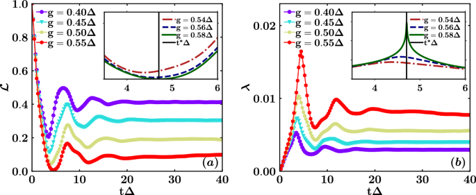
Loschmidt echo \({{\mathcal{L}}}(t)\) (a) and rate function λ(t) (b) as functions of dimensionless time tΔ for different values of the coupling g ∈ [0.40, 0.55]Δ and J = 0, near the critical point, computed through TDVP. The insets provide a zoomed-in view near the transition allowing to identify the critical time t*Δ ≈ 4.7.
To further classify the DQPTs, we study the critical exponent of the rate function of the Loschmidt echo, focusing on the J = −10Δ case and the J = 0 case. The corresponding results are presented in Fig. 9a, b, respectively. We fit the left branch of the data, preceding the peaks, using the function \(\lambda (t)={a}_{L}{\left\vert {d}_{L}-t\right\vert }^{{b}_{L}}+{c}_{L}\) with four free parameters. Subsequently, we fix dL and cL, the coordinates of the peak, for the right branch fitting, which employs the function \(\lambda (t)={a}_{R}{(t-{d}_{L})}^{{b}_{R}}+{c}_{L}\) with two free parameters. In the fit performed for the J = 0 case, we exclude the central points next to the peak.
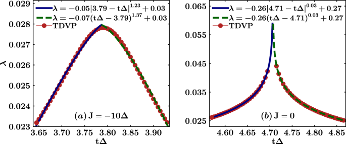
Loschmidt echo rate function λ(t) as functions of dimensionless time tΔ for the two cases J = − 10Δ, g = 0.48Δ (a) and J = 0, g = 0.58Δ (b). The red points represent data computed through TDVP. For each case, we provide fitting functions for both the left branch (blue solid line) and the right branch (green dashed line). The legend indicates the parameter values obtained from the fit.
Our analysis reveals that in the case of J = − 10Δ, the critical exponent b is approximately 1 for both branches. However, in the J = 0 case, the critical exponent b exhibits significantly different behavior, being on the order of 0.03 for both branches. These distinct behaviors point out the significant impact of interactions and entanglement.
As detailed in the Methods Sec. Worldline Monte Carlo method, our model can be mapped by eliminating structured bath degrees of freedom. The resulting effective Euclidean action is characterized by a spin-boson model extended to involve two qubits interacting with the bath, yielding a classical system of spin variables distributed along chains of length β with long-range ferromagnetic interactions. The additional interaction between the two qubits, governed by J, induces short-range interactions between the spin chains. From this perspective, we interpret our resulting critical exponents in analogy with other studies focusing on Ising spin chains and the occurrence of DQPTs. In particular, the case of J = −10Δ can be seen as a system where the short-range interaction between the two chains and the initial qubits’ entanglement are dominant for short times, inducing a quasi-linear critical exponent similar to those observed in short-range Ising chains20. In the J = 0 case, only long-range ferromagnetic interactions are present, with no entanglement between qubits. Interactions between the chains are induced by the coupling to the bath, reducing the critical exponent. As mentioned in the introduction, it has been shown21 that long-range interactions can give rise to DQPTs. However, the exact value of the critical exponent in our case with γ = 2 (BKT), given γ defined by the 1/rγ behavior for long-range interactions, remains unclear. Additionally23, demonstrates that one can obtain a non-linear singularity by changing some parameters in the quench, and22 effectively reduces the critical exponent by considering a random Ising chain.