We have designed Chrysalis to seamlessly integrate into workflows based on SCANPY55 or Squidpy56 Python packages. As such, SCANPY functions are utilised for quality control (QC) and preprocessing for all datasets. Given that Chrysalis assumes that unique tissue compartments are represented by extreme points, stringent QC and outlier removal are important for finding high-quality tissue compartments. During our analyses, SCANPY functions were used to perform QC by first filtering spots based on the unique molecular identifier (UMI) count numbers (pp.filter_cells). The exact cutoff value can be determined individually for samples based on the UMI count distribution and other technical attributes. Genes expressed in less than 10 capture spots (pp.filter_genes) were subsequently discarded. Following that, the gene expression matrix was normalised (pp.normalize_total) and log1p-transformed (pp.log1p) using SCANPY preprocessing functions before subjecting it to further analysis.
Detection of SVGs
PySAL’s57 implementation of the global Moran’s Index (Moran’s I) is used (Supplementary Fig. 17a) to detect SVGs in the gene expression matrix. First, we standardise the preprocessed (normalised and log1p-transformed) expression matrix so that for each capture spot \(i\), the standardised gene expression \({z}_{i}\) can be described as:
$${z}_{i}=\frac{{x}_{i}-\bar{x}}{{\sigma }_{x}}$$
where \({x}_{i}\) represents the expression level of a specific gene at the \(i\)-th capture spot, while \(\bar{x}\) is the mean expression level across all spots and \({\sigma }_{x}\) is the standard deviation of expression levels across all spots. Moran’s I58 can then be formulated as follows:
$$I\,=\frac{n}{{\sum}_{i}{\sum}_{j}{w}_{i,j}}\frac{{\sum}_{i}{\sum}_{j}{w}_{i,j}{z}_{i}{z}_{j}}{{\sum}_{i}{{z}_{i}}^{2}}$$
where \({z}_{i}\) and \({z}_{j}\) are the standardised gene expression levels at spots \(i\) and \(j\), respectively. \(n\) is the total number of spots and \({w}_{{ij}}\) is the spatial weight between spot \(i\) and spot \(j\). Spatial weight \({w}_{{ij}}\) is defined as 1 if spot \(j\) is within the set number of k-nearest neighbours (KNN) of spot \(i\), and 0 otherwise. To evaluate the potential influence of neighbourhood size, we computed Moran’s I statistic with 6, 18, and 36 neighbours (Supplementary Fig. 17b) on the 10x Visium human lymph node sample (for details on preprocessing, see Methods, Human lymph node analysis section). As our results show consistent Moran’s I values regardless of neighbourhood size, Chrysalis uses 6 nearest neighbours by default for computational efficiency, reflecting the hexagonal grid pattern in which Visium capture spots are organised. For analysing Cartesian grid-based technologies (e.g., Stereo-seq, Visium HD) and the in silico data, we used a neighbourhood size of 8. The Slide-seqV2 dataset was analysed with the same neighbourhood size of 8 due to the binning we performed during preprocessing (see Methods, Slide-seqV2 mouse hippocampus analysis section).
Moreover, we also explored alternative spatial autocorrelation statistics to Moran’s I, namely, Geary’s C59. It has been previously reported60 that combining the two metrics can yield better performance, as Geary’s C is more sensitive to local changes. Nevertheless, these two metrics were indistinguishable in our tests using the preprocessed 10x Visium human lymph node dataset (for details on preprocessing, see Methods, Human lymph node analysis section), and therefore we continued with Moran’s I (Supplementary Fig. 17c). To decrease computational runtimes, Chrysalis calculates Moran’s I only for genes that are expressed in at least 5% of the capture spots. This approach does not compromise the identification of spatially variable genes, as demonstrated by the 2D histogram showing that genes exhibiting high Moran’s I values tend to be expressed across wider regions of the tissue (Supplementary Fig. 17d).
To determine the number of SVGs, a rank-order plot is generated by arranging the Moran’s I values for every gene in descending order. This results in a curve characteristic of a power-law distribution (Supplementary Fig. 17e). The inflexion point of this curve, marking the transition from a high-autocorrelation interval to a flatter low-autocorrelation interval, serves as a cutoff point for classifying SVGs. Genes below this inflexion point are omitted, preserving most of the spatial variability in the data while reducing noise. Our findings indicate that in the majority of cases, the inflexion point occurs approximately at the 1000th gene. Consequently, Chrysalis classifies the top 1000 genes as SVGs by default, which are then used for further analysis.
For SVG detection, Chrysalis can also incorporate alternative methods61,62,63,64, which may provide marginal improvements in performance at the cost of increased computational runtimes (Supplementary Fig. 18). To compare the performance of these SVG detection methods to Moran’s I, the 10x Visium human lymph node dataset was preprocessed using SCANPY. SVG detection methods SpatialDE261, SEPAL62, BSP63, and SPARK (SPARK-X)64 were run according to the published guidelines (Supplementary Table S1). Chrysalis was then applied using the top 1000 SVGs assigned by each method (for details on preprocessing, Chrysalis pipeline, and correlation-based validation, see Methods, Human lymph node analysis section). Pearson correlation coefficient was then calculated between the tissue compartments and the cell type deconvolution results.
Low-dimensional embedding
PCA is performed (Scikit-learn65 Python package implementation) on the SVG matrix to identify the main spatial expression patterns. To determine the optimal number of PCs, we conducted multiple tests with varying configurations using the human lymph node dataset (PCs: [6, 10, 20, 40], compartments: 3–24). We calculated a correlation matrix between the cell type deconvolution results and the compartments identified by Chrysalis (see the details in Methods, Human lymph node analysis section) and assessed the average Pearson’s r value of the highest correlating cell type-tissue compartment pairs to evaluate the compartments’ ability to depict the true tissue microenvironments (Supplementary Fig. 19a). Based on this analysis we set the default to 20 PCs, as it sufficiently captured information attributed to the underlying tissue microenvironments.
Morphological feature integration
Chrysalis can incorporate latent feature vectors obtained through deep learning models from H&E images associated with ST measurements. This allows the identification of tissue compartments with unique transcriptional and morphological properties. The generic workflow includes:
1.
Extracting morphological features for each capture spot.
2.
Performing dimensionality reduction on the feature vectors.
3.
Concatenating the morphology-based and gene expression-based components.
4.
Scaling the concatenated components to prevent any issues arising from disparate scales across modalities.
The integrated feature matrix can be subsequently used in Chrysalis to find tissue compartments with archetypal analysis (for details regarding the integration performed for the human breast cancer data, see Methods, Human breast cancer analysis, Morphological feature extraction and integration section).
Tissue compartment inference
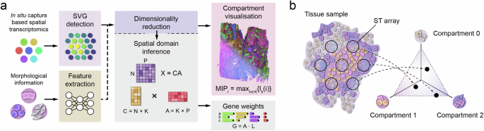
To detect tissue compartments, Chrysalis uses archetypal analysis on the low-dimensional embedding of SVGs. The goal of archetypal analysis is to identify extremal points in multidimensional data, known as archetypes (e.g., tissue compartments), such that any capture spot in the dataset can be represented as a convex combination of these archetypes. This can be interpreted as fitting a multidimensional simplex to the data space with the archetypes representing the vertices of this simplex (Fig. 1b and Supplementary Fig. 5d). Therefore, any observation in the data (i.e.,: each capture spot) can be represented as a mixture of archetypes with a measurable contribution of each archetype to the sample, allowing a comprehensive understanding of the tissue structure.
More formally, let \(X\) be a data matrix of size \(N\times P\), where \(N\) is the number of observations (capture spots) and \(P\) is the dimension of low-dimensional SVG representation (selected number of principal components).
Archetypal analysis aims to find a set of \(K\) archetypes such that the input data matrix \(X\in {R}^{N\times P}\) can be approximated as \(X\approx {CA}\), where \(C\in {R}^{N\times K}\) denotes the coefficient matrix and \(A\in {R}^{K\times {P}}\) denotes archetypes. This approximation is subject to the following constraints:
$$\forall i\in [1…N], {\sum}_{k=1}^{K}{C}_{i,k}=1\wedge {C}_{i,k}\ge 0$$
Where \({C}_{i,k}\) denotes the contribution of \(k\)-th archetype to the \(i\)-th observation.
The process of obtaining matrices \(C\) and \(A\) involves minimising the reconstruction error, measured as the Frobenius norm across all data points formulated as follows:
$${\min } _{C,A}\parallel X-{CA} \, {\parallel }_{F}^{2}$$
Moreover, each observation is approximated as:
$${X}_{i}\approx {\sum}_{k=1}^{K}({C}_{{ik}}\cdot {A}_{k})$$
Upon optimisation, the low-dimensional SVG representation is decomposed into \(K\) archetypes. To obtain archetypical decompositions of SVGs, the PCA loadings can be used as described below. Let \(L\) represent the loadings obtained through PCA decomposition of SVGs. The expression of the individual genes for archetype \(k\) represented by \({E}_{k}\) can be calculated as follows:
$${E}_{k}={A}_{k}\cdot L+\mu ={G}_{k}+\mu$$
where \(\mu\) is the preprocessed mean (normalised and log1p-transformed, for details, see Methods, Chrysalis overview, Data preprocessing section) gene expression vector, and \({G}_{k}\) represents the weights of each gene in the \(k\)-th archetype.
Chrysalis leverages the archetypes Python package implementation of archetypal analysis (n_init = 3, max_iter = 200, tol = 0.001, random_state = 42).
Visualisation
To jointly visualise the tissue compartments, MIP is used. Initially, each archetype \(k\) (tissue compartment) is assigned to a unique colour \({I}_{k}\) in the RGB space, with each colour channel containing values in the range [0, 255]. Following that, linear interpolation is used to assign colours to each capture spot \(i\) for every tissue compartment \(k\). Consequently, the assigned colour values transition between (0, 0, 0), which is assigned to the lowest value in compartment \(k\), and \({I}_{k}\). Given \(K\) tissue compartments, the visualisation colour for a spot \(i\) is determined using MIP as follows:
$${MI}{P}_{i}=({ma}{x}_{k\in K}\{{r}_{k}(i)\},{ma}{x}_{k\in K}\{{g}_{k}(i)\},{ma}{x}_{k\in K}\{{b}_{k}(i)\})\,$$
where \({r}_{k}(i)\), \({g}_{k}(i)\), and \({b}_{k}(i)\) represent the red, green, and blue values for compartment \(k\) at spot \(i\).
In silico ST dataSynthetic ST data generation
To benchmark Chrysalis, we adapted a synthetic ST data generator from prior works20,37. The data generation process follows two main steps:
Cell type abundance simulation along spatial patterns
To simulate cell type abundance, Gaussian process was first used to generate spatial patterns for a 2-dimensional array with Cartesian coordinates corresponding to an arbitrary number of tissue zones in the sample. By tuning parameter eta, the sparsity of the tissue zones was controlled, resulting in sparse (eta = 1.5) and uniform (eta = 1.0) tissue zones. To introduce variability in the spatial coherence of tissue zones, we employed a range of length scale parameter values [4, 10]. Higher length scale values are associated with strongly correlated, spatially coherent variations across the tissue zones, while lower values produce more localised variations, with rapid changes and strong correlations only between nearby points. Detailed parameter values are provided in Supplementary Table S2. A softmax function and min-max normalisation were subsequently applied to the sparse and uniform tissue zones to adjust their scale to [0, 1].
Cell type abundance assignment and expression profile generation relied on annotated input scRNA-seq data. For our benchmarks, we used the Tabula Sapiens38 immune cell atlas. The cell atlas was first subsampled (pp.subsample from SCANPY) to 26 000 cells, on which quality control was performed. We excluded cells with over 20% mitochondrial gene counts and those expressing more than 2500 unique genes. Additionally, cell types represented by fewer than 100 cells and genes expressed in fewer than 10 cells were discarded. After these filtering steps, the resulting cell atlas comprised 17 000 cells spanning 26 unique cell types.
Next, we performed binary assignment of sparse and uniform cell types to tissue zones and patterns. Cell types present in the scRNA-seq input data were randomly assigned to the sparse tissue zones using a binomial distribution function (p = [0.02, 0.04]). For the uniform tissue zones, one cell type per zone was randomly selected.
Following that, we assigned cell types to high or low abundance groups, generating average abundance values for each cell type. This was performed by drawing the abundance values from gamma distributions with different shape parameters for the two abundance groups (shapehigh = 5, shapelow = 3).
We then multiplied the average cell type abundances with the corresponding tissue zones to compute abundance at each location. A noise factor was subsequently added using a log-normal distribution (mean = 0, σ = 0.35) to mimic real tissue variability.
Generation of multi-cell mRNA expression profiles with confounding technical variation
To build the count matrix, we randomly selected cells based on the previously assigned abundance matrix for each location. After that, mRNA abundance across all cell types was aggregated to produce multi-cell mRNA profiles. To introduce technical variation, we first multiplied the counts with a detection rate parameter drawn from a gamma distribution (shape = 5, scale = 1/15). This was followed by calculating a contamination vector introducing counts to each gene by multiplying the average gene counts with contamination fractions drawn from a gamma distribution (shape = 0.03*100, scale = 1/100)). This vector was then applied for genes at every location resulting in a per-location average contamination matrix.
Sequencing depth effects were also modelled by a per location sequencing depth effect (shape = 1*25, scale = 1/25) and a per experiment depth effect (shape = 1*5, scale = 1/5) sampled from two gamma distributions. The count matrix was multiplied with the two sequencing depth effects, and the final counts were then sampled from a Poisson distribution. This was further multiplied by the final contamination counts sampled from a Poisson distribution using the previously calculated per-location average contamination.
To benchmark performance across technical variation, we introduced an alternative approach that keeps the total count number stable irrespective of the fraction of contaminating random counts. Instead of depending on average contamination and sequencing depth values sampled from gamma distributions, we modelled the contamination directly as a fraction of the average count of every gene (\(\gamma\)), with the range of [0.03, 0.09, 0.27, 0.81] across the generated sample set. We further modified the original approach by shuffling the per-location average contamination matrix across genes and spatial locations, replacing the uniform contamination that models only gene-specific variability. Sample-wise sequencing depth effect was also directly specified as a range of fractional values multiplying the synthetic count matrix [1, 0.2, 0.04, 0.008, 0.0016, 0.00032]. The final contamination counts were added to the count matrix after multiplying the original counts by \((1-\gamma )\). For the full range of parameters used in the synthetic data generation process, see Supplementary Table S2.
As the random seed and the tissue zone number parameters are fixed in the technical variation benchmark, the resulting samples share identical spatial patterns and cell type abundance matrices. The difference therefore is only reflected by the increasing amount of technical noise introduced.
To measure the effect of different spatial array sizes, 3 samples were selected from the main dataset and truncated to different spatial dimensions (50\(\times\)50, 25\(\times\)50, 25\(\times\)25) by systematically reducing the spatial arrays’ dimensions by half in each step (Supplementary Fig. 3).
Benchmarking
Calculating low-dimensional embeddings of the benchmarked methods
Before running Chrysalis, we normalised (pp.normalize_total) and log1p-transformed (pp.log1p) the gene expression matrix using SCANPY. We then employed Chrysalis to identify SVGs using Moran’s I with 8 nearest neighbours and selected the top 1000 genes amongst genes expressed in more than 5% of the capture spots. Finally, Chrysalis was used to define tissue compartments using archetypal analysis (number of PCs = 20, number of compartments = number of sparse tissue zones).
To run NSF14 and MEFISTO15, the gene expression matrix was decomposed to a number of factors equal to the number of sparse tissue zones using their respective software implementation pipelines (Supplementary Table S1) after preprocessing the data with SCANPY following the same criteria as for Chrysalis.
For STAGATE27, and GraphST28, the low-dimensional embeddings were extracted after running their respective inference pipelines according to the published guidelines (Supplementary Table S1). This resulted in low-dimensional embeddings with 30 latent features for STAGATE. As GraphST outputs a reconstructed gene expression matrix, we applied a PCA and used an equal number of PCs as sparse tissue zones generated for each synthetic sample. We note that due to excessive computational time, we omitted SpatialPCA from the in silico benchmarks and only evaluated its performance on real-world examples.
Calculating performance metrics
To compare the performance of the tested methods, we first calculated the pairwise Pearson correlation between the sparse tissue zones and the inferred factors or latent features. For each tissue zone, the highest Pearson’s r value was selected. These values were then averaged, representing the overall performance of the models on a single sample.
Human lymph node analysis
We obtained the 10x Visium human lymph node dataset from the 10x Genomics online data repository and preprocessed it using the SCANPY package as described below. First, capture spots containing less than 6000 UMI counts were removed (pp.filter_cells) to filter out low-quality spots. Genes expressed in less than 10 spots were discarded (pp.filter_genes). Next, we normalised (pp.normalize_total) and log1p-transformed (pp.log1p) the gene expression matrix. We then employed Chrysalis to identify SVGs using Moran’s I, selecting genes with at least 0.08 Moran’s I value amongst genes expressed in more than 5% of the capture spots. 997 SVGs above the previously defined Moran’s I threshold were used to construct a low-dimensional representation using the dimensionality reduction step of Chrysalis. Finally, Chrysalis was used to define tissue compartments using archetypal analysis (number of PCs = 20, number of compartments = 8). The included histology image was used to annotate tissue regions.
Validation with cell type deconvolution results and specific marker genes
Correlation with reference data
Cell type deconvolution results were generated with cell2location20 by running the Google Colaboratory notebook provided in the documentation (Supplementary Table S1), using scRNA-seq reference data from the original publication. This single-cell reference was originally obtained by integrating datasets from human secondary lymphoid organs comprising more than 70 000 cells. Correlation coefficients were calculated using the Pearson method to analyse the relationships between the 8 tissue compartments identified with Chrysalis and the inferred abundances of 34 cell types. Subsequently, these coefficients were used to construct a correlation matrix for validating the tissue compartments.
Correlation with marker gene signatures
We explored canonical marker gene signatures of 16 cell types found in the lymph node derived from the CZ CELLxGENE Discover online resource. Using SCANPY’s tl.score_genes function, scores for each of the 16 downloaded gene sets were determined by calculating the difference between their average expression and the average expression of a reference gene set, which was randomly sampled from the total gene pool corresponding to discretised expression levels. Pearson correlation coefficients were calculated, and a correlation matrix was constructed to denote the association between the signature scores and the compartments.
Benchmarking
Calculating low-dimensional embeddings of the benchmarked methods
To run the inference pipelines we used the same procedures described in the In silico ST data, Benchmarking, Calculating low-dimensional embeddings of the benchmarked methods section, with the exception of setting the number of extracted factors (NSF, MEFISTO) to 8 factors. STAGATE and SpatialPCA outputs a low-dimensional embedding with 30 and 20 dimensions, respectively. Therefore we tested those without further processing. For GraphST, we performed PCA on the transformed count matrix and selected the first 20 PCs corresponding to the inflexion point in the cumulative explained variance curve.
Assessment of alternative methods in characterising germinal centres
To benchmark the effectiveness of the low-dimensional representations in characterising the annotated germinal centres, we selected spatial domains (i.e., individual factors from NSF and MEFISTO, embedding vectors from STAGATE, and SpatialPCA, and PCs for GraphST) best describing the annotated germinal centres as described below. First, the low-dimensional representations were min-max normalised to be within the range of [0, 1]. Subsequently, using the germinal centre annotations from the cell2location article20, we calculated the area under the receiver operating characteristic curve (ROC AUC) scores to identify the embedding vectors most representative of the germinal centres. (Supplementary Fig. 4b, c). Following that, the mean Jensen–Shannon distance was calculated between the embedding vector (i.e., domain score) distributions (Supplementary Fig. 4d) for spots labelled as germinal centres and the rest of the sample from 1000 random permutations.
Benchmarking alternative methods with cell type deconvolution results
For the correlation-based benchmark, the unscaled low-dimensional representations were used. Correlation matrices were first built by calculating Pearson correlation coefficients between the 34 cell type abundances from the cell2location reference data and the embeddings. For each cell type, the highest Pearson’s r value was selected, corresponding to the highest correlating embedding vector, and the averages of these values were calculated.
Computational running time
The computational running time of these methods was gauged by measuring execution time starting by reading the dataset up to the point where the low-dimensional representations were calculated (Supplementary Fig. 19b). This measurement was done on a Windows machine using Ubuntu 20.04 LTS via Windows Subsystem for Linux without GPU acceleration (CPU: AMD Ryzen 9 5900HS, RAM: 32 GB, GPU: NVIDIA GeForce RTX 3060 Laptop GPU).
Human breast cancer analysis
The combined 10x Xenium and Visium human breast cancer dataset was downloaded from the 10x Genomics online resource with the corresponding high-resolution H&E. The Xenium dataset contains 167 780 segmented cells with the gene expression data of 313 genes. Cell type annotations of 20 cell types were directly provided by 10x Genomics (Supplementary Fig. 7b).
Co-registration of Visium and Xenium data
To map individual cells from the Xenium section to the Visium data, we first co-registered the two corresponding H&E tissue images. We utilised the image alignment functionality of 10x Genomics’ Loupe Browser, which offers manual landmark-based image alignment. We placed 30 landmarks to create the initial alignment, followed by an algorithmic refinement step relying on the mutual information measured between the two images. Two image registration steps were carried out: one between the post-Xenium H&E and the image captured by the CytAssist machine, and another one between the pre-Visium H&E and the CytAssist image, as the image alignment functionality in Loupe Browser is limited to CytAssist generated image data. Afterwards, affine transformation matrices were exported and used to translate the XY positions of individual cells in the Xenium dataset to the Visium coordinate system (Supplementary Fig. 7c). Cells with centroids outside of the Visium capture spots were omitted and the remaining ones were aggregated for each cell type and assigned to the capture spots (Supplementary Fig. 7d). As there is no one-to-one mapping between the two modalities, spots outside of the Xenium ROI were also removed, retaining 3906 of the original 4992 capture spots.
Mapping pathologist annotations to the Visium dataset
The high-resolution post-Xenium H&E image was assessed and annotated by a trained veterinary pathologist using QuPath66 software. Transformation matrices described in the above paragraph were used to translate the annotation polygons and the spatial coordinate pairs of the Visium dataset to a unified coordinate system. Visium capture spots were subsequently labelled according to their overlap with the annotation polygons (Supplementary Fig. 7a).
Validation with Xenium data
Correlation with reference data
Visium data was preprocessed by normalising (pp.normalize_total) and log1p-transforming (pp.log1p) the gene expression matrix using SCANPY. Once the ground truth data measured with Xenium were added, we discarded low-quality spots containing less than 1000 UMI counts (pp.filter_cells) and genes expressed in fewer than 10 spots (pp.filter_genes) using SCANPY. SVGs were first determined using Chrysalis with the following parameters: minimum Moran’s I = 0.05, genes expressed in > 5% of the total number of capture spots. The detected SVGs were used to construct a low-dimensional representation using the dimensionality reduction step of Chrysalis. Chrysalis was subsequently used to define tissue compartments using archetypal analysis (number of PCs = 20, number of compartments = 8). To examine the relationship between the Xenium reference data and the compartments identified by Chrysalis, a correlation matrix was constructed by calculating Pearson correlation coefficients between these elements.
Marker gene contributions
SVG weights for each tissue compartment were calculated using Chrysalis to assess the importance of breast cancer and myoepithelial marker genes acquired from the original study40.
Assessing cell type composition of tissue compartments
To determine the cell type composition within each tissue compartment, we selected capture spots with domain scores above 0.8. We then aggregated the abundance data of the 20 mapped reference cell types and calculated their respective proportions per compartment.
Benchmarking
To benchmark methods based on their correlation with the Xenium reference data, we used the same procedures described in the In silico ST data, Benchmarking, Calculating low-dimensional embeddings of the benchmarked methods section, with the exception of setting the number of extracted factors (NSF, MEFISTO) to 8 factors. STAGATE and SpatialPCA outputs a low-dimensional embedding with 30 and 20 dimensions, respectively. Therefore we tested those without further processing. For GraphST we performed PCA on the transformed count matrix and selected the first 20 PCs.
Morphological feature extraction and integration
To incorporate morphological information, the spatial positions of capture spots from the Visium sample were first mapped to the 40X magnification post-Xenium H&E slide scan. Transformation matrices were used to translate the spatial positions between the two tissue sections (for details, see Methods, Human breast cancer analysis, Co-registration of Visium and Xenium data section). 3906 image tiles (299 × 299 px) were then extracted (Supplementary Fig. 8a) by marking squares with centroids equal to those of the capture spots and side lengths equal to the capture spot diameters (55 µm). The image tiles were resized to 256 × 256 px, and the pixel values were standardised to be within the range of −1 to 1. The transformed images were used to train a deep autoencoder. The encoder was built using three 2D convolutional layers (kernel size: 3) and a dense layer, all coupled with GELU activation functions. The encoder output (i.e., bottleneck) is a 1-dimensional vector of 512. The decoder contains one dense layer and three 2D transposed convolution layers (kernel size: 3). The first three layers utilised GELU activation functions, while a Tanh activation function was employed for the last layer, resulting in an output size equivalent to that of the input image (pre-trained model is available at Zenodo). The architecture was built and trained using PyTorch67 and PyTorch-Lightning for 100 epochs with a batch size of 1 and learning rate decay using the Adam optimiser. After training, the latent vector for each encoded image tile was collected, resulting in a 2D matrix of 3906 × 512. Next, a PCA was performed on this matrix and the PCs were min-max scaled using scikit-learn’s MinMaxScaler function. Simultaneously, the same operation was applied to the PCs of the SVG expression matrix. The scaled morphology PCs (10) were then concatenated with the SVG expression PCs (20), and the resulting matrix of 30 PCs was subsequently processed with Chrysalis to find tissue compartments (number of PCs = 30, number of compartments = 8).
To demonstrate the benefits of the multimodal approach, we assessed the performance of Chrysalis relying on our pathologist’s annotations (see Methods, Human breast cancer analysis, Mapping pathologist annotations to the Visium dataset). We assigned every spot to the tissue compartment with the highest domain score (Supplementary Fig. 8b). ARI was computed between those compartments and the annotation labels. F1 score was then calculated for every combination of annotations and tissue compartments computed by the gene expression-based and morphology-integrated approaches (Supplementary Fig. 8c). Precision-recall curves for selected annotations were calculated using the respective tissue compartments with the highest F1 score (Supplementary Fig. 8d).
Mouse brain analysisFFPE coronal section processing and benchmarking
The brain section was acquired from the 10x Genomics online repository. Manual annotations were generated by a trained veterinary pathologist using QuPath66 software by assessing the high-resolution H&E image. Visium capture spots were subsequently labelled (Supplementary Fig. 9a) according to their overlap with the annotation polygons.
Capture spots containing less than 3000 UMI counts were omitted (pp.filter_cells), and genes expressed in 10 or fewer capture spots were also removed (pp.filter_genes) using SCANPY. This was followed by a normalisation (pp.normalize_total) and log1p-transformation (pp.log1p) step.
Chrysalis was used to determine SVGs on genes expressed in > 5% of the total number of capture spots. The top 1000 detected SVGs were used to construct a low-dimensional representation using the dimensionality reduction step of Chrysalis, followed by tissue compartment identification (number of PCs = 20, number of compartments = 28).
To run the inference pipelines we used the same procedures described in the In silico ST data, Benchmarking, Calculating low-dimensional embeddings of the benchmarked methods section, with the exception of setting the number of extracted factors (NSF, MEFISTO) to 8 factors. STAGATE and SpatialPCA outputs a low-dimensional embedding with 30 and 20 dimensions, respectively. Therefore we tested those without further processing. For GraphST we performed PCA on the transformed count matrix and selected the first 20 PCs. The output vectors were subsequently scaled to [0, 1].
Following that, the mean Jensen–Shannon distance was calculated between the embedding vector distributions (Supplementary Fig. 9e) for spots labelled with one of the six cortical layers (L1, L2/3, L4, L5, L6) and the rest of the sample from 1000 random permutations.
FF parasagittal section
To process the FF anterior half of the mouse parasagittal brain section, the data was first downloaded from the 10x Genomics online data repository. Manual annotations were acquired from another publication28. Capture spots containing less than 1000 UMI counts were omitted (pp.filter_cells), and genes expressed in 10 or fewer capture spots were also removed (pp.filter_genes) using SCANPY. This was followed by a normalisation (pp.normalize_total) and log1p-transformation (pp.log1p) step.
Chrysalis was used to determine SVGs with the following parameters: minimum Moran’s I = 0.05, genes expressed in > 5% of the total number of capture spots. The detected SVGs were used to construct a low-dimensional representation using the dimensionality reduction step of Chrysalis. Chrysalis was used to define tissue compartments (number of PCs = 20, number of compartments = [8, 12, 16, 20, 24, 28]) and to visualise them (Supplementary Fig. 11b). Based on the results of 28 tissue compartments, the neocortex layers (Compartments 4, 15, 8, 1, and 11) were manually identified. The visual representation of the tissue compartments was examined and directly annotated based on the Allen Mouse Brain Atlas44. Additionally, we performed uniform manifold approximation and projection (UMAP) on the dataset using SCANPY. Chrysalis’s MIP method was used to shade the capture spots to verify the proximity of cortical tissue compartments in the UMAP space (Supplementary Fig. 11c).
Sample integration
The posterior part of the parasagittal mouse brain dataset was downloaded from the 10x Genomics online data repository and preprocessed identically to the anterior sample described above. Data integration was performed with Scanorama68 after the initial normalisation (pp.normalize_total) and log1p-transformation (pp.log1p) of the count matrix for each sample. Following that, Chrysalis was used to calculate SVGs for both samples separately (minimum Moran’s I = 0.20, genes expressed > 10% of the capture spots), and the SVG gene sets were concatenated. This resulted in 1325 SVGs with 675 genes overlapping between the two samples (Supplementary Fig. 12c). The resulting SVG count matrix was used for dimensionality reduction and spatial domain detection by Chrysalis to identify tissue compartments (number of PCs = 20, number of compartments = 10).
Visium HD colorectal cancer analysis
Visium HD data of human colorectal cancer was downloaded from the 10x Genomics data repository. The gene expression matrix corresponding to the 16 × 16 μm rectangle bins was read with SCANPY. Normalisation (pp.normalize_total) and log1p-transformation (pp.log1p) were subsequently performed after filtering out capture spots containing less than 1000 UMI counts (pp.filter_cells) and genes expressed in 10 or fewer capture spots (pp.filter_genes). Chrysalis was used to find the top 1000 SVGs (minimum Moran’s I = 0.05, genes expressed >5% of the bins, number of neighbours for Moran’s I calculation = 8). SVGs were afterwards used to construct a low-dimensional representation using the dimensionality reduction step of Chrysalis. Then, Chrysalis was used to define tissue compartments using archetypal analysis (number of PCs = 20, number of compartments = 28).
Slide-seqV2 mouse hippocampus analysis
Slide-seqV2 data of mouse hippocampus was downloaded using the link provided by the original study6. The count matrix and the corresponding spatial coordinates were read, and the appropriate AnnData data structure was manually constructed with SCANPY. Spatial locations beyond a circle with a radius of 2440 px from the mean XY spatial coordinate pair were removed to discard spots outside of the original ROI. The data was binned into square-shaped bins with a size of 24.4 px to create an evenly spaced array from the randomly dispersed capture beads. Bins containing less than two beads were omitted from further analysis. This was followed by removing capture spots containing less than 100 UMI counts (pp.filter_cells) and genes expressed in 10 or fewer bins (pp.filter_genes) using SCANPY. The count matrix was then normalised (pp.normalize_total) and log1p-transformed (pp.log1p). Chrysalis was used to find SVGs (minimum Moran’s I = 0.05, genes expressed > 5% of the bins, number of neighbours for Moran’s I calculation = 8). SVGs were used to construct a low-dimensional representation using the dimensionality reduction step of Chrysalis. Subsequently, Chrysalis was used to define tissue compartments (number of PCs = 20, number of compartments = 11).
Stereo-seq mouse embryo analysis
Stereo-seq data of mouse embryo cross sections (E9.5, E12.5 – bin 50) were downloaded from the MOSTA: Mouse Organogenesis Spatiotemporal Transcriptomic Atlas data repository. The gene expression matrix in these datasets is tiled up to 25 × 25 μm rectangle bins. HDF files were read with SCANPY, and bins labelled as cavities were removed using the provided annotations. Normalisation (pp.normalize_total) and log1p-transformation (pp.log1p) were subsequently performed. Chrysalis was used to find SVGs (minimum Moran’s I = 0.05, genes expressed > 5% of the bins, number of neighbours for Moran’s I calculation = 8). SVGs were afterwards used to construct a low-dimensional representation using the dimensionality reduction step of Chrysalis. Then, Chrysalis was used to define tissue compartments using archetypal analysis (number of PCs = 20, number of compartments = 24).
Super-resolution tissue compartments with iStar
To demonstrate the compatibility of Chrysalis with super-resolution methods, we used the previously analysed human breast cancer sample generated with the 10x Visium platform. Following the instructions from the iStar documentation, we prepared the data and trained the iStar model. The resulting gene expression matrix predicted gene expression for 1000 SVGs across 472 320 spatial locations derived from the whole-slide image. Using this gene expression matrix as input, we ran Chrysalis with the same settings as for the original data (number of PCs = 20, number of compartments = 8).
Statistics and reproducibility
For the evaluation and benchmarks, Pearson correlation coefficients were computed with the pearsonr function from SciPy’s69 stats module. Jensen–Shannon distance was determined using the jensenshannon function from SciPy’s spatial.distance module. ROC curves and F1 scores were generated using the roc_curve and f1_score functions, respectively, from SciPy’s metrics module. The Adjusted Rand Index, used to evaluate morphological feature integration, was calculated with the metrics.adjusted_rand_score function. Visualisations, including boxplots, violin plots, bar plots, line plots, heatmaps, and others, were created using matplotlib70 and seaborn71.
Reporting summary
Further information on research design is available in the Nature Portfolio Reporting Summary linked to this article.