In this study, station based hourly reported ozone pollutants in ppb extracted from the Air Quality Control Company (AQCC) of Tehran, from 2013 to 2022 for the JJA period is used. The data was extracted for Sharif University Station, because it has the longest data record. The extracted hourly O3 concentration was in ppb, so it was converted to the 8-hour maximum daily average (MDA8). It’s noteworthy to say that ozone is evaluated for 8 h because it reflects cumulative exposure and provides a more accurate assessment of health risks20.
The heat stress analysis is based on meteorological data of temperature and humidity for synoptic Mehrabad Station, obtained from the Iran Meteorological Organization (IRMO) from 1979-2014.2.1.2. Reanalysis and projection data.
In the downscaling model of the study, the predictor data were meteorological variables retrieved from ERA5 reanalysis data. The meteorological variables were selected to predict ozone concentration based on a similar study13. Following this, specific humidity (SH850), temperature (T850), geopotential height (GH850), and vertical as well as horizontal components of the wind (VW850, UW850) were chosen. For this purpose, the aforementioned data was extracted from the European Center for Medium-Range Weather Forecasts dataset. Data was downloaded for the area of study at 850 hPa and for the years between 2013 and 2022 on a daily time scale.
The other predictor for MDA8 ozone pollutant was the ozone concentration in 850 hPa from Copernicus Atmosphere Monitoring Service (CAMS) reanalysis from the European Centre for Medium-Range Weather Forecasts (ECMWF). For ozone projection levels, monthly average ozone data from the BCC-CSM2-MR climate model under the SSP scenario for the time period between 2015 and 2100 and grid type of the study area is downloaded from the USGS database. the BCC-CSM2-MR climate model, models with O3 prescribed from a data set and as part of CMIP6. Hence, there exists a dataset encompassing comprehensive three-dimensional information for both the stratosphere and troposphere. This dataset spans from pre-industrial eras to the current time and extends to the conclusion of the 21st century across different Shared Socioeconomic Pathway (SSP) scenarios21. Therefore, for these kinds of models with no interactive chemistry model, an O3 dataset is provided as part of the Chemistry Climate Initiative (CCM). The CCMI aims to conduct a detailed evaluation of participating models using process-oriented diagnostics derived from observations22. This data was also implemented on a monthly resolution from 2013 to 2022 and also from 2022 to 2100.
The Climate Model Intercomparison Project Phase 6 (CMIP6) models for meteorological parameters in heat index calculation and the ozone projection downscaling model is used. Therefore, the results of a recent study23) are implemented that evaluated the performance of CMIP6 models to select the most suitable model among others in Iran. In this study, 30 models of CMIP6, considering TCR and ECS, were evaluated to investigate temperature spatial distribution and annual trends in Iran with data from Iran’s 51 synoptic stations for the historical period (1980–2014). Results showed that four models, including CanESM5, INM-CM5-0, TaiESM1, and UKESM1-0-LL, have shown the highest performance in estimating the temperature in Iran23). Thus, the Canadian Earth System Model Version 5 (CanESM5) model was used. Besides, note that due to the implementation of the Heat Index (HI) and ozone definitions and concepts, the modeling period focused on the warm months of the year, particularly the June, July, and August (JJA) months.
Analysis
According to the flowchart presented in Fig. 1, this research has been conducted using three data sets, which are detailed in the previous sections. This section outlines the steps and methods used in this research.
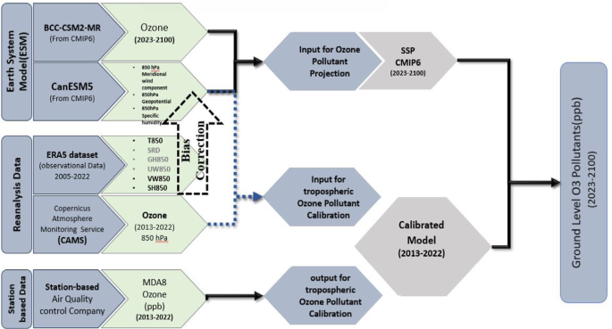
Schematic diagram of the study for ozone projection.
HI calculation
In this study, the NOAA Heat Index (HI) is used to quantify the heat stress concept. Accordingly, the computation of heat index is based on multiple regression analysis that originated from Lans P. Rothfusz24. Rothfusz describes the regression equation as follows (Eq. 1):
$$\begin{aligned} {\text{HI}} & = – {\text{42}}.{\text{379}}+{\text{2}}0.0{\text{49}}0{\text{1523}}*{\text{T}}+{\text{1}}0.{\text{14333127}}*{\text{RH}} – .{\text{22475541}}*{\text{T}}*{\text{RH}} \\ & \quad – 0.00{\text{683783}}*{\text{T}}*{\text{T}} – 0.0{\text{5481717}}*{\text{RH}}*{\text{RH}}+0.00{\text{122874}}*{\text{T}}*{\text{T}}*{\text{RH}} \\ & \quad +0.000{\text{85282}}*{\text{T}}*{\text{RH}}*{\text{RH}} – 0.00000{\text{199}}*{\text{T}}*{\text{T}}*{\text{RH}}*{\text{RH}} \\ \end{aligned}$$
(1)
Where T is temperature in degrees F and RH is relative humidity in percent. HI is the heat index expressed as an apparent temperature in degrees F. If the RH is less than 13% and the temperature is between 80 and 112 degrees F, it has adjustments in its formula. There are four main classifications for HI values according to NOAA, where HI levels between 80 and 90 are in the Caution group, 91–103 are in the Extreme Caution, 104–124 are in Danger group, 125–137 are in Extreme Danger.
As described in Eq. 1, two meteorological factors of temperature and humidity are coupled in the definition of HI. The selected historical dataset was downscaled using a statistical approach and the CanESM5 model for SSP245 and SSP585 CMIP6 scenarios. As the result, the study evaluated the CMIP6-GCM by comparing it to climatic data and then downscaling it using SDSM for the specific location. Then HI is calculated using Eq. 1.
For the parameter selection, the ERA5 dataset was used to determine the effective parameters in ozone forecasting in the period from 2013 to 2022, as well as the bias correction of the ESM model dataset. Thus, first, a regression model was developed to predict ground level observation ozone with T850, GH850, UW850, VW850, and SH850 parameters, as well as ozone obtained from the CAMS dataset. Based on statistical indicators, it was determined that UW850 and GH850 parameters don’t have a special effect on increasing the accuracy and error reduction of the developed regression model. Therefore, they were ignored, and only T850, VW850, and SH850 parameters, along with CAMS ozone, were selected for the next steps. Then these three parameters, extracted from the CanESM5 dataset, were modified based on the ERA5 dataset to develop the final model for projecting surface ozone concentration for the 2023–2100 period. Finally, ozone data from CAMS and three modified parameters (T850, VW850, and SH850) from CanESM5 were used as input and ground-level ozone parameters from Tehran Air Quality Control Company as output to develop a prediction model in the period from 2013 to 2022. The calibrated model by different methods used to predict ground level ozone observations in Tehran by ozone dataset from BCC-CSM2-MR and three modified parameters (T850, VW850, and SH850) from CanESM5 as predictor for the 2023–2100 period.
Statistical downscaling
There are many statistical downscaling approaches presented and compared in different studies26. In our study, according to13 to assess future changes of local ground-level O3, the statistical downscaling framework was based on the Perfect Prognosis (PP) approach and is implemented in the urban area of Tehran City. Perfect prognosis (PP) statistical downscaling uses synoptic meteorology and climatology to simulate regional climate, analyzing the relationship between synoptic scale and regional weather27. In this approach, maximum daily averages 8-hr values (MDA8) is established as the target value.
To generate statistical projections for future climate and emission scenarios, a methodology involved replacing reanalysis predictor data with bias-corrected Earth System Model (ESM) output in Multiple Linear Regression (MLR) models. The focus was on two selected future scenarios, SSP245 and SSP585, during the periods of 2041–2060 and 2081–2100, and with the reference historical period of 2003–2019. This approach aimed to highlight the local changes in ozone (O3) levels anticipated under the influence of projected climate change, providing an understanding of the potential impacts on atmospheric composition in the specified timeframes.
For prediction of station-based scenarios, various machine learning functions were used. The models encompass Artificial Neural Network (ANN), ensemble method (ENS), Regression linear (REG), Support Vector Machin algorithm (SVM), Gaussian Process Regression (GPR), and M5 tree-based machine learning methods (M5tree). For this purpose, the predictor was chosen as ozone obtained from the CAMS (2013–2022) database and meteorological parameters from ERA5, and the predictand was station base MDA8 ozone concentrations. Therefore, the aforementioned machine learning techniques with the specified predictand and predictors resulted in the modeling of SSP scenarios of CMIP6 ozone levels. The machine learning model for ozone pollutant was trained using a 5-fold cross validation method, with 70% data for calibration and 30% for validation.