The software was developed using MATLAB 2023a using Windows 10.
Simulations
The simulation of the single molecule data was done using SMIS2.1, running in MATLAB 2022 in Windows 10. Imaging parameters were chosen to represent the local single-molecule microscope.
For the image generation, we used the following properties for the simulation. The difference between 2D and 3D simulations are the “simul_3D” value, which was 1 for 3D simulations and the diffusion environment used for the particles.
To generate a simulated diffusion environment in both 2D and 3D, an initial widefield image of T. brucei was utilized. The image underwent processing in Fiji, including Gaussian blurring with a width of 0.5, followed by edge detection and binarization using the Otsu method. The “Fill Holes” command was then applied to obtain a closed shape of the parasite, where the value 1 represented the parasite, and 0 represented the outer area. This binarized image was saved and imported into MATLAB to create a 3D diffusion environment.
In MATLAB, the “erode” command was employed to systematically reduce the size of the shape at its edges. This erosion process was repeated four times until the remaining shape resembled the center of the original parasite image. Each iteration of erosion was saved and used to construct additional layers of the 3D object. The original binarized image was placed in the center, with four layers added on top and four layers added below to mimic a three-dimensional trypanosome. Voxel values of 1, representing the parasite, in contact with the outside (value of 0) were assigned a value of 2 to denote them as membrane voxels. The resulting model was saved in a dataframe format suitable for use in the SMIS software.
Cell culture and cell line generation
T. brucei strain Lister 427 were cultivated at 37 °C, 5% CO2 in HMI-9 (Hirumi’s Modified Iscove’s medium-9) containing 10% heat-inactivated fetal bovine serum.
Sample preparation and imaging
Thickness-corrected coverslips were placed in coverslip racks made from Teflon and cleaned 2 times using 2% Hellmanex-II solution by incubating them for 10 min in an ultrasonic water bath (Elmasonic P, Elmasonic) using 100% power, a frequency of 37 kHz at room temperature. Coverslips were then washed using ddH2O and stored in ddH2O until use. On the day of the experiment, two coverslips per sample were dried using an air stream and placed in a clean petri dish. For one experimental day, 1 × 10⁷ cells were harvested by centrifugation at 1500 × g for 10 min at room tempreature. The supernatant was removed, and the cells resuspended in 1 ml of vPBS (PBS supplemented with 10 mM glucose and 46 mM sucrose, pH 7.6). Cells were washed 3 times with 1 ml of vPBS at 800 × g for 2 min, followed by resuspension in 100 µl vPBS, containing 1 nM Atto643-NHS (ATTO-TEC), and incubation for 5 min on ice. The dye labels the variant surface glycoprotein coat of the parasites. Following incubation with the dye, the cells were washed 3 times with 1 ml of vPBS at 800 × g for 5 min at 4 °C. Finally, the cells were resuspended in 20 µl vPBS and stored on ice. As trypanosomes are highly mobile parasites, they need to be immobilized for imaging. For this, a mixture of 8-arm PEG-VS (2.5 µl of 50 mM solution, Sigma-Aldrich) was used together with hyaluronic-acid functionalized with an SH group (8–10 kDa, DS 40%, 3 µl of 25% solution, AG Groll15). Additionally, 1 µl of 1:100 diluted latex beads (BD Biosciences) of 6 µm diameter were used as a spacer to guarantee equal spacing of the coverslips. As a buffer 2 µl of vPBS and 2 µl of cell suspension were mixed and added onto a coverslip. A second coverslip was placed on top, and a weight of 90 g was applied to the sample. The coverslip sandwich was then centrifuged for 1 min at 1500 × g to collect the trypanosomes at the lower coverslip.
Imaging was done at 37 °C on an inverted widefield microscope (Leica DMI6000B) with an Olympus 100 × oil immersion objective (HCX PL APO 100 × 1.47 OIL CORR TIRF) and a dichroic filter (zt405/514/633rpc, 670, Chroma). Fluorescence was excited using a laser beam (Hübner Photonics) at 640 nm with a power of 3 kW/cm2. Pulsed illumination was controlled using an acusto-optical tunable filter AOTF to reach illumination times of 9 ms or 36 ms at frame rates of 100 Hz or 25 Hz for 2D and 3D, respectively. Either 2500 or 5000 frames were acquired. Image acquisition was performed using an Andor iXon697 with a gain of 150, running in cropped mode with a ROI of 120 × 120 pixel. The acquisition process was controlled using MicroManager 2.0.
For calibration of the 3D astigmatic approach, TetraSpeck™ (ThermoFisher Scientifc) beads were immobilized using the PEG-HASH hydrogel and z-stacks with 10 nm step size were acquired.
Image processing
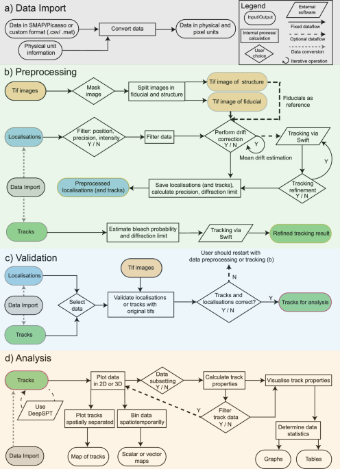
Calibration image stacks of fluorescent beads were processed in SMAP to determine the astigmatism using a spline fit. The resulting calibration file was used for z-position determination in the experimental image data. For this, the batch mode of SMAP was used. The localizations were then loaded into ThirdPeak, and a manual mask was applied to only include trypanosome cells. Next, localizations were filtered by their precision (σXY ≤ 100 nm, σZ ≤ 200 nm) and corrected for drift using a mean-shift approach. The resulting localizations were saved as CSV files for tracking analysis by swift. The data were loaded into ThirdPeak to refine the tracking by adjusting the expected displacement and bleach values accordingly. Tracking was optimized by iterating the tracking process until the expected displacement between 2 loops differed less than 5%. These optimized tracks were then loaded into ThirdPeak for further analysis.
During optimization, the tracking process converged the expected displacement value for the two-dimensional simulation to 217 nm, for the three-dimensional simulations to 290 nm and for the experimental data to 170 nm due to the immobile particles present in the experiment.
Tracking using swift
For the tracking of the localization data, we used swift (Endesfelder et al., manuscript in preparation, beta-testing repository http://bit.ly/swifttracking), a tracking algorithm relying on Markovian statistics and initial starting parameters. It operates in three stages, the first main tracking stage in which a global optimal linking solution should be found, followed by the pruning stage. During this stage, less likely connections are removed in dense localization regions. In the last postprocessing stage, potential errors that occurred in the main tracking stage can be corrected (swift 0.43 manual).
Statistics and reproducibility
The experimental data of living, immobilized trypanosomes consist of 40 and 35 cells, respectively for the 2D and 3D case. These cells were acquired from three technical replicates on the same day. For the 2D experiments, 8696 tracks were used for analysis, in the 3D case, 15,020 tracks were analyzed. For the simulations, one file for each condition (2D and 3D) was generated and 4025 tracks and 9590 tracks were analyzed in the 2D and 3D case, respectively.
Functions in the softwareHeatmap generation
As biological data is inherently noisy, generating heatmap by binning single-molecule localizations and tracks into larger areas can reveal processes that might just be hidden inside the noise itself. For this, the data range of the tracks is used, and the x, y, z coordinates are placed into respective bins, depending on the user-defined size. Additionally, the user can choose to change the temporal binning by increasing the number of time windows, thereby splitting the data also in the temporal space. This feature detects the directionality of the tracks, the velocity of particles and the number of localizations in each bin.
Jump distance
The jump distance describes the Euclidean distance of a particle between two consecutive timepoints in 1D, 2D or 3D, depending on the choice of the user. For one dimension:
$${{d}}_{n}={x}_{t}-{x}_{t+1}$$
where d describes the distance between two time points in one of the dimensions, xt the positional argument of one dimension at timepoint t and xt+1 the positional argument of one dimension at timepoint t + 1.
For two dimensions:
$${{d}}_{2D}=\sqrt{{({x}_{t}-{x}_{t+1})}^{2}+\,{({y}_{t}-{y}_{t+1})}^{2}}$$
For three dimensions:
$${{d}}_{3D}=\sqrt{{({x}_{t}-{x}_{t+1})}^{2}+\,{({y}_{t}-{y}_{t+1})}^{2}+\,{({z}_{t}-{z}_{t+1})}^{2}}$$
Mean jump distance
The mean jump distance is calculated per track from the jump distances calculated above by:
$$\bar{d}=\frac{1}{n}\sum _{i=1}{{\rm{d}}}_{i}$$
Net track distance
The net track distance describes the distance between the first and last localization of a particle:
$${{d}}_{{net}}={x}_{1}-{x}_{n}$$
Total track distance
The total track distance describes the complete length of a trajectory:
$${d}_{{tot}}=\sum _{i}{{d}}_{i}$$
Basic confinement ratio
The confinement ratio (Rconf) divides the total track length by the net distance. If Rconf Rconf > 1, the track is confined.
Diffusion coefficient estimation by jump distance distribution
Estimating the diffusion coefficient from the 1D jump distance distribution is a robust way of calculating this property under the assumption of Brownian motion, especially when having short tracks, as a fit to the mean-squared displacement becomes less reliable. To retrieve the diffusion coefficient, fitting a normal distribution onto the jump distance distribution of one dimension can be performed. The standard deviation from this fit can then be retrieved and by the Einstein–Smoluchowski equation the diffusion coefficient can be calculated by:
$$D=\frac{{\sigma }^{2}}{\varDelta t}$$
where D is the diffusion coefficient, σ is the standard deviation and \(\varDelta t\) the respective timeframe. This however only determines the overall diffusion coefficient and can not distinguish between different populations.
Diffusion coefficient estimation by cumulative jump distance distribution
To distinguish between multiple populations, an analysis using the cumulative jump distance distribution can be performed by fitting the integrated distribution in accordance with Weimann, Klenerman18 for 2D:
$$P\left({r}^{2},\Delta t\right)=\,{\int }_{0}^{{r}^{2}}p\left({r}^{2}\right)d{r}^{2}=1-{e}^{-\frac{{r}^{2}}{4D\Delta t}}$$
for one species, and if multiple species are present, the sum is used:
$$P\left({r}^{2},\Delta t\right)d{r}^{2}=\mathop{\sum }\limits_{J=1}^{m}\frac{{f}_{j}}{4{D}_{j}\Delta t}{e}^{-\frac{{r}^{2}}{4{D}_{j}\Delta t}}$$
For 3D data, the following applies:
$$P\left({r}^{3},\Delta t\right)=\,{\int }_{0}^{{r}^{3}}p\left({r}^{3}\right)d{r}^{3}=1-{{\rm{e}}}^{-\frac{r3}{6D\Delta t}}$$
Mean jump distance population distribution
The mean jump distance population distribution is determined by smoothing the histogram of the mean jump distances with a variable kernel filter and determining the maxima in the smoothed data. The maxima are then used in a minimal least squared approach to fit the data with Gaussian populations.
Diffusional confinement ratio
To determine if a particle is confined, an extended ratio in comparison to the basic confinement ratio is possible. The diffusional confinement ratio of a particle is determined by fitting the mean squared displacement with a confined diffusion model:
$${MSD}={R}^{2}* \left(1-{{\rm{e}}}^{-4D\frac{1}{\bar{{R}^{2}}}}\right)+{offset}$$
, where R is the radius of confinement and D the local diffusion coefficient.
Volume calculations
Volume calculations are performed on the total volume the tracks confine. Two options are available, the convex hull, that forms a convex bounding box around the track data, while the alphaShape approach will fit a tight bounding box around the track data.
Jump angle
The angle δ between two vectors, or essentially three points of a single track is calculated as:
$$\delta ={\tan }^{-1}{||}\left({axb}\right)-\left(a\cdot b\right){||}$$
with a and b being the two vectors, respectively.
Additional code packages
We further include major features of the following repositories, if necessary, extending their features for 3D analysis and handling (sparse) track data.
• MSDAnalyzer:n https://github.com/tinevez/msdanalyzer/tree/master
• TIFFStack: https://de.mathworks.com/matlabcentral/fileexchange/32025-dylanmuir-tiffstack
• Mean-Shift-Drift-Correction: https://github.com/frankfazekas/Mean-Shift-Drift-Correction
• Peak finding and measurement: https://de.mathworks.com/matlabcentral/fileexchange/11755-peak-finding-and-measurement-2019?s_tid=srchtitle
• TrackIt: https://gitlab.com/GebhardtLab/TrackIt
• Jump Distance Analysis: https://github.com/rmenssen/JDD_Code
• DeepSPT: https://pubmed.ncbi.nlm.nih.gov/38352328/
• HDBScan: https://github.com/Jorsorokin/HDBSCAN
Reporting summary
Further information on research design is available in the Nature Portfolio Reporting Summary linked to this article.