The Resuscitation Science Center (RSC) of Emphasis at the Children’s Hospital of Philadelphia (CHOP) Research Institute conducts preclinical research, assessing risk factors for, and testing novel therapeutics to treat, neurological injury in animal models. All animal procedures were approved by the CHOP Institutional Animal Care and Use Committee (IACUC) and were conducted in strict accordance with the NIH Guide for the Care and Use of Laboratory Animals and all authors complied with the ARRIVE guidelines. From 2017–2023, 905 animal studies were conducted across a range of translational neurological injury models (51.0% cardiac arrest, 17.9% cardiopulmonary bypass, 15.8% traumatic brain injury, 6.5% carbon monoxide toxicity, 4.2% hydrocephalus, 3.9% congenital heart disease, 0.7% neonatal hypoxia). Animals ranged in age from newborn to 120 days, corresponding to a weight range of ~ 1 to ~ 40 kg. For all experiments, anesthesia was induced via intramuscular injection of ketamine (~ 40mg/kg), buprenorphine (~ 0.02mg/kg) and atropine (0.06mg/kg) for ~ 2kg swine, ketamine (~ 20mg/kg) and buprenorphine (~ 0.02mg/kg) for 4kg-10kg swine, or ketamine (~ 20mg/kg) and xylazine (~ 2mg/kg) for 30-40kg swine. After intubation, inhaled isoflurane is delivered and weaned down from 2% to minimize hemodynamic impact while ensuring a surgical plane of anesthesia by the absence of response to toe pinch. At the conclusion of the experiment, euthanasia is humanely performed utilizing 2-4mEq/kg of potassium chloride administered intravenously. From these experiments, raw data types collected include single measure, repeated measures, time series, and imaging. To facilitate analyses utilizing these heterogeneous data types, the development of a custom data framework was required. Design considerations for this framework included rapidity of processing, near-full automation, adaptability to accommodate potential future data modalities, and embedded review checkpoints to guarantee accuracy of reported data.
The developed data framework encompasses a custom file structure, data collection systems that support investigational monitoring, data processing pipelines that feature data warehousing infrastructure, tailored ETL methodology and architecture, and a visualization platform developed to handle diverse data types across disparate experimental models in a preclinical research setting. To clarify the classification terminology used, “data type” refers to the category of data being collected (“single measure”, “repeated measures”, “time series”, or “imaging”). “Data modality” refers to groups of recorded “data elements”. If the data modality is “Arterial Blood Gas”, a data element is a measured variable within the modality (e.g., “pH”). The “experimental model” refers to the general injury or therapeutic model. The “cohort” refers to a specific study within that experimental model. Lastly, the “subject” refers to an individual experiment, classified by the subject’s unique identifier, which combines the experimental date in the format “YYMMDD” and the number assigned to the animal by the vendor (e.g., “210813_1745”). These naming conventions facilitate multileveled organization and comparative analysis.
File structure
A standardized, hierarchical file structure was implemented to organize the collection, processing, and integration of heterogeneous, longitudinal data types within and across diverse experimental models (Fig. 1). Our team collaborated with the CHOP Research Institute Arcus Library Science Team (H.C., C.D.) to design the file structure.
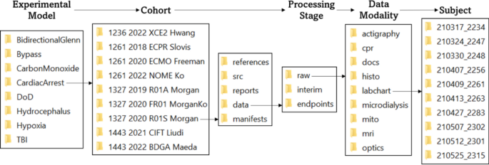
File Structure Diagram: This diagram demonstrates hierarchical organization of the file structure by classifier (experimental model, cohort, subject), processing stage, and data modality. This nested structure facilitates the storage of metadata within the file’s path name, which is more efficient than accessing legend files for downstream data integration and requires no manual updating or quality review. The organization of this file structure allows data to be queried by classifier, processing stage, and data modality, and provides space for the storage of cohort-specific documentation and analysis files.
The file structure described below is hierarchically organized using the classifiers “experimental model”, “cohort”, and “subject”. Each experimental model is identified by a unique name that reflects the model (e.g., “CardiacArrest” for cardiac arrest, “TBI” for traumatic brain injury). To date, twenty-two unique cohorts are contained within the “CardiacArrest” directory. The syntax for cohort directory naming is a combination of the CHOP IACUC protocol number, the year of the first experiment, a unique four-character alphanumeric cohort identifier, and the principal investigator’s last name (e.g., 1261 2022 NOME Ko). Many data modalities are shared by cohorts within the same experimental model. Protocolized data type storage across different experimental models and cohorts enables comparative, cross-sectional data element analyses. Within each cohort directory, data at various stages of processing are contained within a “data” folder. In addition to housing raw experimental data types, the file structure within this folder features designated directories for downstream data processing that facilitates workflow tracking to monitor the processing status of each data modality. Specifically, “raw”, “interim”, and “endpoints” folders indicate the processing status of each data type, and ensures that only processed, quality-reviewed data is integrated and transferred to various locations for sharing, visualization, and further analysis.
Alongside the “data” folder, each cohort directory also contains a “manifest”, “src”, “reports”, and “references” folder. The “manifest” folder contains cohort-wide, automatically-generated sheets, summarizing the data collection and processing status of each data modality (see “Manifest Generation”). The “src” folder contains code and other supporting material for cohort-specific analyses and the “reports” folder contains the results generated by these analyses. Lastly, the “references” folder contains reference material related to the cohort’s experimental design.
Data types and data collection
Diverse, multimodal, preclinical data types are collected during each experiment. Data that are acquired once per subject are referred to as “single measure” data. “Repeated measures” data are acquired at multiple timepoints per subject. These timepoints may be predefined or change from subject to subject. “Time series” data are sequences of data indexed at successive, equally-spaced points in time. A distinction between repeated measures data and time series data is that intervals between repeated measures data are often irregular and at the time scale of hours to days. Finally, the “imaging” data type describes spatial data (greater than one dimension) that may yield data types that are single measure, repeated measures, or time series. Standardized collection instruments were tailored to support specific data types and collection environments and are further described below.
Single measure data
For each experiment, single measure data including demographic information about the subject, the monitoring and data collection techniques used during the experiment, any medications or interventions administered to the subject, and qualitative and quantitative characteristics of the experimental protocol are collected. Examples of collected single measure data include species, sex, date of birth, experimental group, and types of anesthesia administered. The collection of these data allows full understanding of all aspects of an experiment, which is essential to analysis and interpretation of collected physiological data. Single measure data may also be associated with a timestamp; this includes experimental outcomes data that may occur at different experimental timepoints depending upon survival duration. Timestamped, single measure data elements implemented within the platform include quantitative assessments of collected tissue samples (e.g., density of microglia staining in cortical tissue, brain tissue water fraction). Timepoint collection permits cross-sectional analysis of the association of the outcome metric with time and experimental period. Collection tools and methodology of use for single measure data are described below.
Case report forms (CRFs)
CRFs are used in clinical trial research to protocolize collection of patient data and facilitate reporting of this data to sponsoring institutions30. We have translated this data collection practice to preclinical research to standardize collection of data types including experimental protocol characteristics and physiological measurements during experiments. For each subject, three unique CRFs are used to record qualitative and quantitative information during the experiment: the “Anesthesia Record”, “Code Leader”, and “Neuro-Optical Monitoring CRF”.
The “Anesthesia Record” records all experimental, therapeutic, and surgical interventions as well as administration quantities of anesthetic and other drugs. Additionally, hemodynamic and ventilation parameters are manually recorded every 5–10 minutes to ensure the welfare of the animal. Sharing of this document with CHOP’s Department of Veterinary Resources (DVR) is mandated by the United States Department of Agriculture (USDA) to ensure humane treatment of each subject.
The “Code Leader” document is used to record clinically relevant information during the injury and/or therapy portion of the experimental protocol. For instance, the Code Leader document is used during the resuscitation portion of an experiment designed to compare the efficacy of different resuscitation techniques or technologies. During this portion of the experiment, the Code Leader document is used to record the timing of vasopressor administration and defibrillation attempts, as well as “clinical” observations.
Lastly, the “Neuro-Optical Monitoring CRF” is used for recording observations with precise timestamping, focusing on experimental and physiological parameters that may affect cerebral perfusion or neuro-optical monitoring signal quality. All three documents are scanned and uploaded into the subject’s folder within the cohort’s “docs” folder at the conclusion of the experiment. Experimentally relevant single measure and repeated measures data are then manually entered into a customized electronic data capture software.
Electronic data capture software
REDCap (https://projectredcap.org/software/) is a customizable, browser-based, metadata-driven electronic data capture software commonly used in translational research for the collection of single measure and repeated measures data types31,32. REDCap “Arms” are constructs that allow study events to be grouped into a sequence. In our implementation, each “Arm” in the REDCap database represents an experimental cohort and is named using the cohort naming convention (see “File Structure”). “Instruments” are the individual data capture forms that prompt the user for data entry. Our REDCap instruments contain single measure data collection, including subject characteristics (e.g., “Demographics”, “Monitoring”, “Tissue Collection”), as well as data specific to experimental periods (e.g., “Baseline”, “Asphyxia”, “Acute Survival”). Subject characteristics include data collection checklists that are used to track the collection and usability of various measurement modalities (see “Manifest Generation”). When a new cohort is implemented in the REDCap database, only the instruments relevant to that experimental model are selected, with the ability for cohort-level customization. This reduces empty fields and creates a streamlined data entry process.
Biological sample collection characteristics
Single measure data related to stored biological samples are entered into Freezerworks (Dataworks Development, Mountlake Terrace, WA, USA) software. This includes information about the sample, the collection protocol, and its location within the center’s freezer system. The Freezerworks database was designed to categorize samples by cohort and experimental model for compatibility with other in-house data collection systems and processing pipelines.
Assessment of mitochondrial respiration
Mitochondrial respiration is a metric of the oxidative respiratory capacity of the mitochondria and is assessed at a single experimental timepoint from fresh tissue sampled at euthanasia. Significant reduction in respiratory capacity has been associated with adverse functional neurological outcomes33. High-resolution respirometry is used to measure mitochondrial respiration in brain tissue homogenate in an Oxygraph-2k (Oroboros Instruments, Innsbruck, Austria). Additions of complex-specific substrates and inhibitors allow for the assessment of the integrated respiratory capacities of oxidative phosphorylation (OXPHOS) and the electron transport system (ETS). Key data points of interest include the oxidative phosphorylation capacity of complex I (OXPHOSCI) alone and the convergent capacity of complexes I and II (OXPHOSCI+CII), assessment of the leakiness of the mitochondrial membrane, maximal convergent non-phosphorylating capacity of complexes I and II through the electron transport system (ETSCI+CII), ETS capacity through complex II alone (ETSCII), and ETS capacity through complex IV alone (ETSCIV). To normalize quantitative respiration values for mitochondrial content, samples are also assessed for citrate synthase (CS) activity using a commercially available kit, Citrate Synthase Assay Kit CS0720 (Sigma-Aldrich, St. Louis, MO, USA). Raw respirometry data files (.dld) produced by the Oxygraph-2k must be viewed in Oroboros DatLab software and then manually exported as a numerical data table (.csv) to a designated “mito” processing directory in the “raw” data folder where they are later queried by a custom MATLAB (MathWorks, Natick, MA, USA) script for automated processing of respirometry values.
Histopathological quantification
Histopathological quantification of collected tissue samples yields single measure data that will be subsequently discussed in the “Imaging” section.
Repeated measures data
Repeated measures data are captured in “repeated instrument” forms within REDCap, as well as in .csv data tables generated from analyses of biological samples and bedside imaging. Collection tools and methodology of use for repeated measures data are described below.
Electronic data capture software
The custom REDCap database stores repeated measures data (e.g., “Blood Gasses”, “Cardiac Outputs”) utilizing “repeating instruments” to capture all instances of collection, without having to first specify the number of instances. These “repeating instruments” are experimentally timestamped and are later aligned with time series data during the “interim” processing stage to provide additional physiological context.
Cerebral microdialysis quantification
Interstitial fluid from cerebral tissue is invasively collected using a 70 Microdialysis Catheter (M Dialysis Inc., Stockholm, Sweden). The collected dialysate fluid contains metabolites that may be used to characterize neurological injury. Cerebral microdialysis samples are analyzed on the ISCUSflex Microdialysis Analyzer (M Dialysis Inc.). The reagent kit used analyzes the samples for levels of glucose (mg/dL), lactate (mM), pyruvate (µM), and glycerol (µM). Data from the analyzer is exported via USB hard drive and viewed using ICUpilot (M Dialysis Inc.) software, then downloaded as a Microsoft Excel (Microsoft Corporation, Redmond, WA, USA) spreadsheet, which is later queried for experimental time-alignment in the “interim” processing stage.
Venous and arterial blood gas analysis
Blood gas analysis measures the amounts of dissolved gases (oxygen and carbon dioxide), acidity (pH), electrolyte and metabolite concentrations, and co-oximetry from a collected blood sample. Blood gas values from venous and arterial whole blood samples are measured by a GEM Premier 5000 (Werfen, Barcelona, Spain) blood gas analyzer at numerous predefined timepoints for each cohort, manually recorded in the “Code Leader” CRF, and entered into the repeating REDCap instrument, “Blood Gasses”. Each measurement set of blood gasses is entered into a new instance of the repeating instrument within the REDCap entry for the subject and is thus able to be individually queried during the “interim” processing stage.
Cardiac output measurement
Cardiac output is the product of heart rate and stroke volume, measured in liters per minute (L/min). Values are measured by an Agilent V24CT Patient Monitor (Agilent Technologies, Santa Clara, CA, USA) at numerous predefined timepoints, manually recorded in the “Code Leader” CRF, and entered into the repeating REDCap instrument, “Cardiac Outputs”. Each measurement of cardiac output is entered into a new instance of the repeating instrument within the REDCap entry for the subject. These data later undergo subject-specific integration during the “interim” processing stage.
Protein and metabolite quantification
Mass spectrometry of blood serum or plasma samples collected throughout an experiment yields protein and metabolite data that grant a window into the dynamic environment of the proteome and metabolome, respectively. From these data, biomarkers (either protein products or metabolites) of interest may be analyzed over the course of recovery, or as a point of comparison for different groups34,35. Plasma biomarkers are analyzed through the Penn Medicine Human Immunology Core (HIC) using Simoa® (Quanterix Corp., Billerica, MA, USA) assay kits. The HIC compiles assay plate results into an Excel spreadsheet. A custom MATLAB script extracts biomarker data from corresponding spreadsheets, renames data points, and saves these data in .csv files. The .csv files are then imported into R (R Foundation for Statistical Computing, Vienna, Austria) where statistical analysis is performed. Results are saved as .csv files in the subject’s folder within the “interim” directory, along with individual .png files for the generated figures. These data later undergo subject-specific integration during the “interim” processing stage.
Imaging
In many cases, imaging data are collected at numerous experimental timepoints and thus are deemed a repeated measures data type. The unique types of imaging data collected will be elaborated on in the “Imaging” data type section due to heterogeneity and complexity.
Time series data
Several physiological time series data elements are collected throughout each experiment. The collection frequency and period vary by collection instrument. Collection hardware and software for time series data are described below.
Hemodynamic and other physiological waveforms
PowerLab (ADInstruments, Sydney, Australia) hardware modules collect physiological time series data at 1000 Hz. For compatibility with PowerLab, the physiological monitors used must have the capability to export their waveforms as analog output voltage signals. LabChart (ADInstruments, Sydney, Australia) physiological data analysis software centralizes these waveforms and allows the export of all physiological data in one LabChart data file (.adicht) on the same synchronized time axis. Examples of these physiological waveforms include capnography, rectal temperature, and invasively-measured arterial blood pressure. Additionally, cyclic measurements may be derived from waveforms with cyclic features associated with the cardiac or respiratory cycle. Examples of this include the diastolic and systolic pressure calculations from the aortic pressure (AoP), right atrial pressure (RAP), and pulmonary artery pressure (PAP) waveforms, and the end-tidal carbon dioxide (EtCO2) measurement from the capnography waveform. Coronary perfusion pressure (CoPP) is calculated as the difference between the diastolic AoP and diastolic RAP values. These calculated waveforms are then saved and exported distinctly from their derivative waveforms. Calculated waveforms combining two different raw waveforms (e.g., CoPP) are uniquely possible in the preclinical setting and have informed numerous studies on the physiological effects of CPR33,36,37,38,39.
The LabChart .adicht file is read and maintained in its native form for some analyses while the data is divided by experimental periods and down-sampled for other analyses. During down-sampling, each variable is averaged into 15-second (15-s) epochs to strike a balance between information density and ease of data export and visualization. These down-sampled time series data are used for low-resolution waveform analysis during the “raw” processing stage.
Cardiopulmonary resuscitation (CPR) chest compression mechanics
During CPR, a ZOLL R-Series Advanced Life Support Automated External Defibrillator (ZOLL Medical Corporation, Chelmsford, MA, USA) with CPR quality monitoring capabilities is used to record compression mechanics data such as depth, rate, and release velocity. These time series data are exported from the hardware as an .ful file and are viewed in and exported from RescueNet Code Review (Zoll Medical Corporation) software as an .xml document. These time series data are time-aligned with the “CPR” experimental period during the “interim” processing stage.
Actigraphy
The activity level of the subject is measured using an attached accelerometer. This provides an assessment of normal activity as an indicator of neurological impairment following injury. Accelerometer data is collected using a USB Accelerometer X16-1E (Gulf Coast Data Concepts, LLC, Waveland, MS, USA) and is logged on a battery-powered unit that holds 2–3 days of accelerometer data. This data is then downloaded as a .txt file for further “raw” processing and subject-level integration during the “interim” processing stage.
Electroencephalography
A two-channel differential electroencephalography (EEG) montage is used to record EEG waveforms between C3-P3 locations on the left hemisphere, and C4-P4 locations on the right hemisphere, according to the 10–20 system40. EEG waveforms are captured at a sampling rate of 256 Hz on a clinical bedside monitoring device, CNS-100R (Moberg Research, Ambler, PA, USA). This device is manually time-synchronized during each recording session. Recording sessions are exported and translated from their proprietary data format into a .mat data file for import into MATLAB for further processing and alignment with other time series data during the “interim” processing stage.
Neurometabolic optical monitoring (NOM)
Continuous, non-invasive, diffuse optical monitoring of cerebral hemodynamics is conducted using an investigational research instrument that has been previously described41. This research instrument combines the techniques of frequency-domain and broadband diffuse optical spectroscopy (FD-DOS and bDOS, respectively) and diffuse correlation spectroscopy (DCS) via a non-invasive optical sensor that is secured to the animal’s forehead. FD-DOS quantifies cerebral tissue optical scattering and absorption properties from which the tissue concentration of oxy-, deoxy-, and total hemoglobin and cerebral tissue oxygen saturation (StO2) may be derived at a sampling rate of 10 Hz. Using bDOS in conjunction with FD-DOS significantly increases spectral sampling and permits additional quantification of changes in the tissue concentration of water, lipid, and cytochrome c oxidase. bDOS data may be acquired at 1 Hz and is temporally interleaved with FD-DOS and DCS. DCS measures relative changes in cerebral blood flow at a sampling rate of 20 Hz.
Raw NOM waveforms include measured amplitude and phase with respect to modulation frequency, source wavelength and source-detector separation from FD-DOS, absorption spectra from bDOS, and normalized temporal intensity autocorrelation curves and intensities for each detector from DCS. This raw data is imported into MATLAB for further processing during the “raw” processing stage. During “raw” processing, theoretical models of light propagation in tissue are used to numerically derive the value of physiological parameters. NOM-derived physiological parameters are integrated with other physiological time series during the “interim” processing stage. It is important to note that derived physiological parameters vary based on model selection; this poses a challenge to multi-institution data aggregation. Data standardization and optimal model selection are ongoing areas of research in diffuse optics.
Imaging data
Imaging may yield data that are single measure, repeated measures, or time series. We discuss this data type separately due to its unique storage and processing considerations. Imaging data varies in size and type based on modality, dimensionality, number of frames (single image vs. video), and resolution. Raw imaging data are stored in various databases and present unique accessibility challenges compared to the other collected data types. Collection tools, storage platforms, and methodology of use for imaging data are described below.
Magnetic resonance imaging (MRI)
MRI data is acquired using a 3T Tim Trio (Siemens Medical Solutions USA, Malvern, PA, USA). During each MRI session, several individual scan sequences are performed and stored on the scanner under the subject’s identifier. Sequences include anatomical (e.g., T1, T2) and functional imaging (e.g., SWI, DTI, MRS, ASL, BOLD)34,35. Scan data is stored as .dicom files. The scanner is outfitted with a Flywheel (Flywheel Software, San Francisco, CA, USA) “reaper” that moves data from the scanner to Flywheel. Flywheel is a biomedical research data management platform for imaging and associated data. The scanner reaper is configured in a push setup, such that when imaging sessions are completed, the reaper collects the imaging files and pushes them to a Flywheel receiver which distributes them to specific folders in Flywheel. Once in Flywheel, .dicom files are viewable with Flywheel’s web-based image viewer platform. All files are downloaded for “raw” processing and further analysis. Derived categorical and numerical parameters from neuroimaging include presence, location, and size of neuroimaging abnormalities and location and value of spectroscopic analytes. These values are integrated by cohort during the “interim” processing stage. Standardization of derived parameters remains ongoing.
Histology
Numerous tissue samples are collected at the time of euthanasia for histologic analysis of cellular injury and functional impairment34,36. Sampled organs include the brain, heart, and kidney. Tissue samples are formalin-fixed, paraffin-embedded, and sectioned at 5–10 µm for chromogenic and immunofluorescent staining. Images of stained tissue sections are taken on a DMi8 (Leica Microsystems, Wetzlar, Germany) microscope using a FLEXCAM C1 (Leica Microsystems) color camera at 20 × magnification. Images are then exported as .tiff files into ImageJ (https://imagej.nih.gov/ij/), where they are deconvoluted using the “H DAB” function. Thresholding is applied only to the “Colour 2” output to measure positive antibody expression. The preset “Measure” function is used to obtain the area, mean, minimum pixel value, and maximum pixel value for each image. Images and associated .csv files containing quantitative data are stored in a custom histology file architecture where they can be queried for subject-level integration during the “interim” processing stage.
Contrast-enhanced ultrasound (CEUs)
CEUs data is acquired using both a clinical ultrasound scanner (Acuson Sequoia; Siemens Medical Solutions USA) and a research ultrasound scanner (Vantage 256; Verasonics Inc., Kirkland, WA, USA)42,43,44. For the clinical ultrasound scanner, video clips or “cineloops” of clinically relevant timepoints during contrast perfusion are manually saved by the sonographer to the scanner’s internal storage as .dicom files. After the study, the .dicom files are copied to an external USB hard drive. For the research ultrasound scanner, scanning with the probe populates the local machine memory with radio frequency (RF) signal data. The data is asynchronously transferred to a host controller computer via direct memory access according to programmatic requests from custom software written in-house. Once on the host controller, the data is temporarily stored within internal random-access memory (160 GB capacity), and then saved in parallel threads to an internal hard drive storage (28 TB capacity). The RF data can then be processed into images for further visual or computational analysis during “raw” processing. Derived quantitative values are integrated by subject during the “interim” processing stage.
Data processing
A custom data integration and processing pipeline was developed for time synchronization, quality review, and dissemination of collected data. A flow chart demonstrating the functionality of the three data processing stages (“raw”, “interim”, and “endpoints”) can be found in Fig. 2. The pipeline is executed on a subject-by-subject basis during the “raw” and “interim” processing stages, while “endpoints” processing is conducted at the cohort-level. The “raw”, “interim”, and “endpoints” stages populate the corresponding folders of the “data” directory in the file structure (see “File Structure”). This framework provides a standardized, modular system to incorporate novel data types that are a crucial aspect of preclinical research.
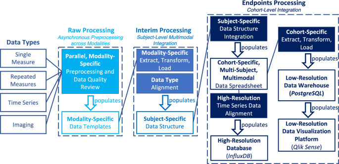
Processing Stage Flowchart: This flowchart demonstrates the functionality of each of the three data processing stages (“raw”, “interim”, “endpoints”). The primary role of each stage is visualized; modality processing during “raw”, subject-integration during “interim”, and cohort-integration during “endpoints”. Data can be traced from raw collected data type to the databases and data visualization platform. It is important to note that the “Imaging” data type represents the quantitative data derived from image files. Raw imaging data is stored in a Flywheel database.
Raw processing: asynchronous preprocessing across modalities
The pipeline starts in the “raw” processing stage with preprocessing and the autonomous and manual data quality review of disparate data types within a flexible file architecture. The “raw” processing stage is composed of three substages. In the first substage, data collection and processing occurs in dedicated modality-specific subdirectories within the “raw” directory. Distinct space allocation for each modality permits asynchronous and parallel data processing across disparate laboratories and personnel, which minimizes bottlenecks.
The second substage of the “raw” processing stage is data quality review. Autonomous data quality criteria are applied and verified by manual data quality review by trained laboratory personnel.
In the third substage, a standardized data template and pipeline import adapter is developed for each data modality for integration with other modalities. Each data template includes subject identification, modality-specific data elements, a time axis (if applicable), and a reference timepoint used to align the time axis to experimental periods. The pipeline import adapter is developed in collaboration with data modality experts to map quality-reviewed data into the standardized data template. Effort is ongoing to incorporate file monitoring to automatically trigger appropriate raw processing substages when all required files are detected.
Interim processing: subject-level multimodal integration
Time synchronization and intra-subject data consolidation occur in the “interim” processing stage. A subject-specific data structure is created to store all aligned and time-synchronized data modalities as the pipeline advances. This data structure includes metadata describing the animal and experimental characteristics and associated data directories. The data structure is populated from each modality’s standardized data templates (created during the “raw” processing stage). For each modality, a dedicated ETL script is developed for import into the data structure.
Time series data that has been experimentally aligned and down-sampled into 15-s epochs during the “raw” processing stage is imported into the subject’s data structure. These modalities include hemodynamics and other physiological parameters, NOM, CPR performance, and EEG data. Next, single measure and repeated measures data are imported and aligned with the corresponding experimental period and respective 15-s epoch. These modalities include REDCap, microdialysis, mitochondrial respirometry, serum biomarkers (proteins and metabolites), and derived imaging metrics data. This integrated data is exported as a tabular .csv file, classified as the “summary” file to the subject’s folder in the “interim” directory, along with the subject’s data structure.
Endpoints processing: cohort-level integration
The “endpoints” processing stage performs cohort-level multimodal data integration and incorporates the extract, transform, and loading of data into the PostgreSQL (PostgreSQL Global Development Group, Berkeley, California, USA) data warehouse for Qlik Sense (Qlik, King of Prussia, PA, USA) dashboard visualization and into the InfluxDB (InfluxData Inc., San Francisco, CA, USA) high-resolution database for downstream machine learning applications. High-quality, multimodal subject data is compiled into a single data sheet for each cohort. The data sheet is two-dimensional with columns containing all measured data elements as well as identifiers for subject, experimental period, and period-specific time, and rows containing incremental data samples. This data sheet is populated from the individual subjects’ tabular .csv files located in the subject’s folder in the “interim” directory and saved in the subject’s folder in the “endpoints” directory where it is queried for further data warehousing.
Extract-transform-load (ETL) pipeline
The cohort-specific, multi-subject, multimodal data spreadsheets are used to populate the high-resolution database (InfluxDB) and the low-resolution data warehouse (PostgreSQL), which ultimately populate the Qlik Sense dashboard. Methodology and architecture related to high-resolution data preparation, the cohort-specific ETL pipeline, and the data visualization dashboard (Qlik Sense) design are presented below.
High-resolution data preparation and import
An InfluxDB database was created to store high-resolution (100 Hz) time series data (F.M., L.S., F.T.) and support preclinical predictive model development. Metadata saved during manual quality review of time series waveforms is applied to high-resolution time series data. Single measure and repeated measures data are then time-aligned with the quality-reviewed, high-resolution time series data. Cohort-level integration is performed and high-resolution, multimodal data .csv spreadsheets are generated for import into InfluxDB.
Low-resolution data warehousing
An ETL-based data warehousing approach is used to integrate data from multiple experimental models into a single, standardized data warehouse (Fig. 3). Here, the ETL is implemented in Python (Python Software Foundation, Wilmington, DE, USA) and loaded into a PostgreSQL data warehouse. The data warehouse compiles data from REDCap instruments, manifest files, summary files, and the Freezerworks database. These data are stored in tables that are related using the unique identifier of each subject. This enables the search and modification of each data modality separately and facilitates dynamic and selective loading into the Qlik Sense dashboard.
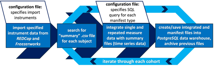
Cohort-Specific Extract, Transform, Load (ETL) Flowchart: This flowchart demonstrates the functionality of the ETL script used for manifest file creation and low-resolution data warehouse (PostgreSQL) data population. Configuration files specify the SQL queries to be used for each data type’s manifest as well as which instruments should be integrated from REDCap and Freezerworks for each cohort. The script iterates through each cohort, then each subject, searching for its “summary” data file. This file’s data is then combined with the single and repeated measures data pulled from REDCap and Freezerworks to generate manifest files that are formatted for, and saved to, the PostgreSQL data warehouse. All previous manifest files are stored as backup files for redundancy and version tracking in the file structure.
REDCap integration
The ETL pipeline extracts data from REDCap using customized application programming interface (API) requests. Relevant REDCap instruments were identified and include “Demographics”, “Monitoring”, “Tissue Collection”, “Resuscitation”, and “Baseline” single measure instruments and “Blood Gasses”, “Cardiac Outputs”, and “ECMO” repeated measures instruments. A configuration file containing this list of instruments was used to extract instrument-specific data from REDCap into a dedicated table within the PostgreSQL data warehouse.
REDCap fields containing multiple choices are concatenated into a single field. Repeat instances are concatenated for ease of storage. Additional transformations are performed, including the creation of tables to associate the REDCap “Arm” names (e.g., cohort names) with the subjects within the cohort, the extraction of the experimental period names from each cohort, and the creation of one master “group” column which combines the various experimental groups (e.g., “sham”, “control”) from each cohort. This transformed data is then loaded into the PostgreSQL data warehouse and designated tables for each REDCap instrument are created.
Freezerworks integration
The ETL pipeline extracts data from Freezerworks using the Freezerworks API request and the unique subject identifiers in each cohort from the associated “interim” folders. Information pertaining to each subject’s biological sample collection is combined into a summary file for each cohort and then into a “master” summary file containing all the cohort’s summary files for upload into the PostgreSQL data warehouse.
Manifest generation
Manifests are tabular records that summarize data modality availability and processing status for each subject across a cohort. Manifests are created by applying logical transformations to inputs including the summary “endpoints” data sheets (see “Endpoints Processing”) and modality collection checklists that are entered into REDCap during the experiment. The output is a categorical variable with the following allowable values and corresponding definitions: −1, data collection not marked complete; 0, data not collected; 1, data collected but not quality-reviewed; and 2, data collected and quality-reviewed.
Logic for identifying the presence of data and determining data availability and processing status is saved in SQL queries. These SQL queries are then run in PostgreSQL using a Python script to populate the tabular “manifest” which is then exported as a .csv file in the “manifest” file directory and saved in the PostgreSQL data warehouse in a dedicated table. Exception logic in the Python script ensures that errors in the data, missing data, and incorrect column naming are identified and recorded without causing a termination of the script’s run.
Workflow automation
The migration of processed data into the PostgreSQL data warehouse is automated to ensure updated data access and an accurate reflection of data availability and processing status.
The ETL Python script was developed and version-controlled using a GitHub (Microsoft Corporation, Redmond, WA, USA) repository. GitHub is a widely used online software development platform that enables storage, tracking, collaborative development, and publishing of software projects. This ETL script is packaged into a single deployable executable using Docker (Docker, Inc., Palo Alto, CA, USA). Docker is a platform for the creation and management of containers. Containers are packaged executables that contain source code, in this case, the ETL Python script, and operating system dependencies that are required to run the source code in any environment. A Dockerfile, which serves as the guidelines to build a Docker image, was developed, and a Docker image was subsequently generated.
A Docker container, which is a running instance of the Docker image is executed daily by Kubernetes (Linux Foundation, San Francisco, CA, USA). Kubernetes is a container-orchestration tool that facilitates the management of the Docker container.
The GitHub directory containing the ETL Python script and Docker container specification script is monitored by Red Hat Quay (Red Hat Software, Raleigh, NC, USA) for any modifications. Red Hat Quay is a container registry that interprets the container specification script and builds, analyzes, and distributes Docker images. When code changes are committed to GitHub, Red Hat Quay automatically detects the commit and triggers the build of a new Docker image.
Once Red Hat Quay generates a Docker image, an “instance” of this container is scheduled to run daily on a Kubernetes cluster. A .json configuration file is imported into Kubernetes, which specifies execution schedule, the location of the image, and the minimum central processing unit (CPU) and memory requirements, amongst other settings. Kubernetes subsequently automates the execution of the ETL script to ensure the PostgreSQL data warehouse is updated daily. The steps of the workflow automation pipeline are demonstrated in Fig. 4.
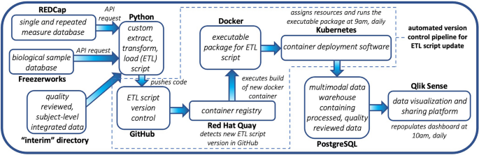
Workflow Automation Pipeline: This pipeline illustrates how components of the data framework are automatically updated when changes are made to the ETL script and how the PostgreSQL data warehouse and Qlik Sense database are automatically updated every day. Changes made to the ETL Python script are pushed to GitHub and detected via Red Hat Quay, triggering a rebuild of the Docker container. Kubernetes deploys the Docker container daily which causes the PostgreSQL data warehouse to be updated. The Qlik Sense dashboard is also updated daily.
Data visualization dashboard
Compiled data streams within the PostgreSQL data warehouse are imported into Qlik Sense, a data discovery, visualization, and export tool. Qlik Sense Enterprise is a commercial web applet that has been made accessible within our institutional network. Customized data visualization dashboards were developed to empower users to explore relevant selections of data, quickly visualize cross-sectional time series data, and perform summary analytics.
PostgreSQL database credentials were provided to Qlik Sense to permit direct query and import of data tables. Specifying table associations within Qlik Sense results in the joining of tables to create a single consolidated table with all unique data fields that may be ubiquitously queried by the subject identifier. Table associations and identifiers are visually depicted in Fig. 5. A built-in scheduling tool within Qlik Sense performs a daily query of the data warehouse and refreshes the consolidated data table.
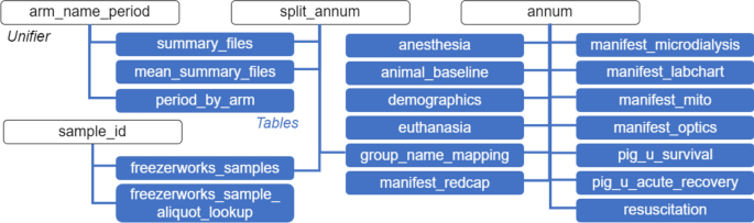
Qlik Sense Dashboard Table Associations: This diagram displays all of the associated tables imported into Qlik Sense and the “unifiers” used to associate them (“arm_name_period”, “split_annum”, “annum”, “sample_id”). “annum” is a subject-level identifier comprised of the experiment date in the format “YYMMDD” and the number assigned to the animal by the vendor. Similarly, “sample_id” is a sample-level identifier that is comprised of the date of biological sample collection in the format “YYMMDD” and the number assigned to the animal by the vendor. “split_annum” is a subject-level identifier that is only comprised of the number assigned to the animal by the vendor. This is used to link data from Freezerworks to data from other sources because the date of biological sample collection, which is tied to Freezerworks data, is not always the same as the experiment date. “arm_name_period” is a cohort-level identifier comprised of the CHOP IACUC protocol number, the year of the first experiment, a unique four-character alphanumeric cohort identifier, and the principal investigator’s last name (e.g., 1261 2022 NOME Ko).
The design of the Qlik Sense dashboard, including featured data fields and layout, was iteratively proposed and reviewed by research team members to ensure broad utility. The final dashboard features a landing page which centralizes data selection filters, graphical display pages which summarize selected data, a tabular page depicting the status of data processing within selected subjects, and a summary data table that permits export of all selected data. Images and further explanations of the dashboard pages are included in the “Supplementary Materials” section.
Personnel
To develop and manage a data framework like the one described presently, several key personnel roles are required. First, a bioinformatician oversees data entry and the addition of new data types and cohorts, and designs new front-end data acquisition systems. This role serves to liaison between the experimental team and the data integrationist. A data integrationist is needed to architect an automatically-updated database, manage all API requests, and develop a custom ETL pipeline. Lastly, a project manager guides the framework, communicating directly with principal investigators to ensure that the data needs of the lab are being met. This person will ensure that the data framework is designed to answer the research questions of interest. To maintain objectivity and avoid bias, the member of the bioinformatics team that performs data quality review (the only qualitative portion of the data framework) is always blinded to the experimental group of the subject they are reviewing.