The dataset of this study was extracted from drugs.com28, which is publicly available in the UCI Machine Learning “Drug Review Dataset (Drugs.com)” repository. The medication review dataset contains 215,063 patients’ sentiments (text) about the medication they used, along with a score from 1 to 10 (numerical) that patients have registered as well as the condition of the medications (text)28. The methodology diagram of this study is illustrated in Fig. 1.
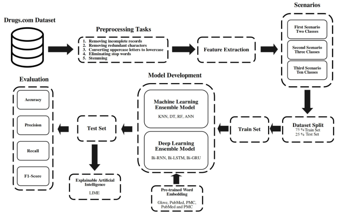
Workflow diagram illustrating the steps performed in this study.
Data preprocessing
In this study, NumPy and NLTK libraries were used to perform preprocessing tasks on medication review texts. This stage had five steps as: (1) removing all incomplete records, (2) removing the redundant punctuation marks and characters from all texts, (3) converting uppercase letters to lowercase letters in all instances of the dataset, (4) deleting the stop words because they were frequently present in the texts and did not provide us with the helpful information in terms of performance, and (5) using Snowball Stemmer to remove the suffixes of the words in the dataset and find their roots. After fully preprocessing, 213,869 samples were remained.
Extracting features from texts
After preprocessing phase, a clean and consistent dataset was created. ML and DL models are not able to work directly with texts. So, texts should be converted to vectors of numbers. This study utilized BoW and word embedding techniques to extract features from texts. BoW is a simple way to count the number of repetitions of words and an easy-to-use technique for converting texts to vectors for classification models47.
Word embedding is a new method to represent any word using a vector of numbers such that each number in the vector represents one latent feature of the word, and the vector represents different latent features of the word48. Word2Vec is a neural network-based word embedding technique. This method comprises three layers: input, hidden, and output. The Word2Vec method consists of two structures, Skip-Gram (SG) and Continuous BoW (CBOW)48. Furthermore, pre-trained word embedding, including Glove in the general domain, and PubMed, PMC, and combined PubMed and PMC in the clinical domain were considered in this study for DL models49,50.
Study design
Three scenarios were implemented in this study. In the first scenario, the scores of the medication reviews dataset were divided into two classes: Negative (for the scores less or equal to 5) and Positive (for the scores greater than 5). In the second scenario, the scores were divided into three classes: Negative (for the scores less than 5), Neutral (for the scores 5 and 6), and Positive (for the scores greater than 6). Eventually, in the third scenario, the dataset scores of this study were considered from one to ten for each medication review.
Dataset split
This study used Hold-Out cross-validation to split patients’ medication review dataset51. According to this method, the dataset was randomly divided into two training and testing sets, so 75% of the dataset was considered for training (160,093 samples) and 25% for testing (53,776 samples).
Prediction models
Nine common models of ML, DL, and ENS with different theoretical backgrounds, including KNN, DT, RF, Artificial Neural Network (ANN), Bidirectional Recurrent Neural Network (Bi-RNN), Bidirectional Long Short-Term Memory (Bi-LSTM), Bi-GRU, Machine ENS learning (ML_ENS), and DL_ENS52,53,54,55,56,57, were developed to predict patients’ sentiment and rate scores. All proposed ML algorithms in this study are described in detail in Appendix A.
DL algorithms depend on activation functions and loss functions during their learning process. By utilizing these functions and updating the weights, the models are trained to make predictions. Rectified Linear Unit (ReLU) is a type of activation function that is used in neural networks to introduce the property of non-linearity to them, and help them learn complex patterns and predict more accurately55. This function sets negative values of input to zero, while leaving positive values unchanged55. The mathematical equation of the ReLU activation function is as follows:
$$\:f\left(x\right)={max}\left(0,x\right)$$
(1)
Where \(\:x\) represents the input value.
Sigmoid is an activation function that takes any inputs and transforms them into output values in the range of 0 to 1 in neural networks55. The sigmoid function is commonly used in binary classification tasks55. The following equation shows how the sigmoid activation function works:
$$\:\sigma\:\left(x\right)=\frac{1}{1+{e}^{-x}}$$
(2)
Where \(\:\sigma\:\) represents the sigmoid function, and \(\:e\) represents Euler’s number.
Softmax is an activation function that converts numbers or logic to probabilities. Softmax’s output is a vector of probabilities for the possible outcomes55. It is used to normalize the output of neural networks. Unlike the sigmoid activation function, it is commonly utilized for multivariate classification tasks55. The following equation shows how the softmax activation function works:
$$\:S{\left(\overrightarrow{z}\right)}_{i}=\frac{{e}^{{z}_{i}}}{{\sum\:}_{j=1}^{K}{e}^{{z}_{j}}}$$
(3)
Where \(\:S\) is softmax, \(\:\overrightarrow{z}\) devotes input vector, \(\:{e}^{{z}_{i}}\) standard exponential function for input vector, \(\:K\) shows the number of classes in multivariate classification, and \(\:{e}^{{z}_{j}}\) means standard exponential function for output vector.
The loss function is a function that is calculated to evaluate the models’ performance in modeling the dataset55. In other words, it measures the difference between the predicted and actual target values55. The following equation represents how binary log loss is calculated:
$$\:Binary\:Log\:Loss\:=\:-\frac{1}{N}{\varSigma\:}_{i=1}^{N}{y}_{i}log{\widehat{y}}_{i}+\left(1-{y}_{i}\right){log}\left(1-{\widehat{y}}_{i}\right)$$
(4)
Where \(\:{y}_{i}\) shows actual values, and \(\:{\widehat{y}}_{i}\) shows model predictions.
Another loss function that is used for multivariate classification is categorical cross-entropy loss55, which is calculated as follows:
$$\:Categorical\:Cross-Entropy\:Loss=\:-{\sum\:}_{j=1}^{K}{y}_{j}{log}\left({\widehat{y}}_{j}\right)$$
(5)
Where \(\:{y}_{i}\) shows actual values, and \(\:{\widehat{y}}_{i}\:\)shows model predictions55.
RNN is a type of ANN which used in text, speech, and sequential data processing54,55. Unlike feed-forward networks, RNNs have a feedback layer where the output of the network and the next input are fed back to the network55. RNNs have internal memory, so they can remember their previous input and use their memory to process sequential inputs. Long Short-Term Memory (LSTM) and GRU are among the RNN algorithms in which the output of the previous layers is used as input to the subsequent layers54. LSTM and GRU, in their architecture, solve the vanishing gradient problem that occurs in RNN54,55. Bi-RNN, Bi-LSTM, and Bi-GRU algorithms have a two-way architecture55. These three algorithms move and learn in two directions (forward and backward) in a progressive and regressive way55.
The output of Bi-RNN is:
$$\:p\left(\left.{y}_{t}\right|{\left\{{x}_{d}\right\}}_{d\ne\:t}\right)=\varphi\:\left({W}_{y}^{f}{h}_{t}^{f}+{W}_{y}^{b}{h}_{t}^{b}+{b}_{y}\right)$$
(6)
Where
$$\:{h}_{t}^{f}=\:tanh\:({W}_{h}^{f}{h}_{t-1}^{f}+\:{W}_{x}^{f}{x}_{t}+\:{b}_{h}^{f})$$
(7)
$$\:{h}_{t}^{b}=\:tanh\:\left({W}_{h}^{b}{h}_{t-1}^{b}+\:{W}_{x}^{b}{x}_{t}+\:{b}_{h}^{b}\right)$$
(8)
That \(\:{x}_{t}\) denotes the input vector at the time \(\:t\), \(\:{y}_{t}\) is the output vector at the time \(\:t\),\(\:\:{h}_{t}\) is the hidden layer at the time \(\:t\), \(\:f\) means forward, \(\:b\) means backward, and \(\:{W}_{y}\), \(\:{W}_{h}\), and \(\:{W}_{x}\) denote the weight matrices that connect the hidden layer to the output layer, the hidden layer to the hidden layer, and the input layer to the hidden layer, respectively. \(\:{b}_{y}\) and \(\:{b}_{h}\) are the bias vectors of the output and hidden layer, respectively55.
In the following, the calculation process of Bi-LSTM is explained:
$$\:{f}_{t}=\sigma\:({W}_{f}\left[{h}_{t-1},{x}_{t}\right]+{b}_{f}$$
(9)
$$\:{i}_{t}=\sigma\:({W}_{i}\left[{h}_{t-1},{x}_{t}\right]+{b}_{i}$$
.
$$\:{\stackrel{\sim}{C}}_{t}=tanh\:({W}_{c}\left[{h}_{t-1},{x}_{t}\right]+{b}_{c}$$
(11)
$$\:{C}_{t}=\:{f}_{t}{C}_{t-1}+\:{i}_{t}{\stackrel{\sim}{C}}_{t}$$
(12)
$$\:{o}_{t}=\sigma\:({W}_{o}\left[{h}_{t-1},{x}_{t}\right]+{b}_{o}$$
(13)
$$\:{h}_{t}=\:{o}_{t}\:{tan}h\left({C}_{t}\right)$$
(14)
Equations (9–14) are the equations of the forgotten gate, input gate, current state of the cell, memory unit status value, output gate, and hidden gate, respectively. The \(\:b\) and \(\:W\) denote the bias vector and weight coefficient matrix55. \(\:\sigma\:\) shows the sigmoid activation function55.\(\:\:{x}_{t}\) denotes the input vector at the time \(\:t\) and \(\:{h}_{t}\) is the hidden layer at the time \(\:t\)55. The output of Bi-LSTM is:
$$\:{y}_{t}=g({V}_{{h}^{f}}{h}_{t}^{f}+\:{V}_{{h}^{b}}{h}_{t}^{b\:}+\:{b}_{y})\:$$
(15)
Where
$$\:{h}_{t}^{f}=g({U}_{{h}^{f}}{x}_{t}+{W}_{{h}^{f}}{h}_{t-1}^{f}+{b}_{h}^{f})$$
(16)
$$\:{h}_{t}^{b}=g({U}_{{h}^{b}}{x}_{t}+{W}_{{h}^{b}}{h}_{t-1}^{b}+{b}_{h}^{b})$$
(17)
That \(\:{y}_{t}\) is the output vector at the time \(\:t\),\(\:\:f\) means forward, \(\:b\) means backward, and \(\:V\), \(\:W\), and \(\:U\) denote the weight matrices that connect the hidden layer to the output layer, hidden layer to hidden layer, and input layer to hidden layer, respectively54.
The calculation process of Bi-GRU is:
$$\:{z}_{t}=\sigma\:{(W}_{xz}{x}_{t}+{W}_{hz}{h}_{t-1}+{b}_{z})$$
(18)
$$\:{r}_{t}=\sigma\:{(W}_{xx}{x}_{t}+{W}_{hr}{h}_{t-1}+{b}_{r})$$
(19)
$$\:{\stackrel{\sim}{h}}_{t}=\:tanh\:{(W}_{xh}{x}_{t}+\:{r}_{t}^\circ\:\:{h}_{t-1}{W}_{hh}+\:{b}_{h}$$
(20)
$$\:{h}_{t}=\:(1\:-\:{z}_{t})^\circ\:\:{\stackrel{\sim}{h}}_{t}\:+\:{z}_{t}^\circ\:{h}_{t-1}$$
(21)
Where \(\:W\) is the weight matrix, \(\:{z}_{t}\) shows update gate, \(\:{r}_{t}\:\)represents the reset gate, \(\:{\stackrel{\sim}{h}}_{t}\) shows reset memory, and \(\:{h}_{t}\) shows new memory. \(\:{x}_{t}\) denotes the input vector at the time \(\:t\), and \(\:b\) is the bias vector55. The output of Bi-GRU is:
$$\:{h}_{t}=\:{W}_{{h}_{t}^{f}}{h}_{t}^{f}+\:{W}_{{h}_{t}^{b}}{h}_{t}^{b}+\:{b}_{t}$$
(22)
Where
$$\:{h}_{t}^{f}=GRU({x}_{t},\:{h}_{t-1}^{f})$$
(23)
$$\:{h}_{t}^{b}=GRU({x}_{t},\:{h}_{t-1}^{b})$$
(24)
That \(\:GRU\) is the traditional GRU computing process, \(\:f\) and \(\:b\) mean forward and backward, respectively, and \(\:{b}_{t}\) is the bias vector at the time \(\:t\).
Supposing \(\:h\) is equal to Eq. (6) for Bi-RNN, Eq. (15) for Bi-LSTM, and Eq. (22) for Bi-GRU, and the parameters are: the number of these models units is \(\:150\), the number of units in the first fully connected layer is \(\:n=128\), and the number of units in the second fully connected layer is \(\:z\), given a single time step input:
$$\:{o}_{1}=ReLU\left({W}_{1}h+{b}_{1}\right)$$
(25)
$$\:{o}_{2}=\:{f}_{i}\left({W}_{2}{o}_{1}+{b}_{2}\right)$$
(26)
Where Eqs. (25, 26) are the equations of the first fully connected layer with ReLU activation and the second fully connected layer, respectively. \(\:{f}_{i}\) could be sigmoid as Eq. (2) for the first approach, and it could be softmax as Eq. (3) for the second and third approaches. The \(\:{b}_{1}\) and \(\:{b}_{2}\) denote the bias vectors and \(\:{W}_{1}\) and \(\:{W}_{2}\) denote weight coefficient matrices.
By knowing \(\:t=1\), and \(\:{f}_{i}\) is sigmoid, we have these proposed algorithms:
$$\:Bi-RNN=\:Sigmoid\left({W}_{2}\left(ReLU\left({W}_{1}\left(\varphi\:\left({W}_{y}^{f}{h}_{t}^{f}+{W}_{y}^{b}{h}_{t}^{b}+{b}_{y}\right)\right)+{b}_{1}\right)\right)+{b}_{2}\right)$$
(27)
$$\:Bi-LSTM=\:Sigmoid\left({W}_{2}\left(ReLU\left({W}_{1}\left(g\right({V}_{{h}^{f}}{h}_{t}^{f}+\:{V}_{{h}^{b}}{h}_{t}^{b\:}+\:{b}_{y}\left)\right)+{b}_{1}\right)\right)+{b}_{2}\right)$$
(28)
$$\:Bi-GRU=\:Sigmoid\left({W}_{2}\left(ReLU\left({W}_{1}({W}_{{h}_{t}^{f}}{h}_{t}^{f}+\:{W}_{{h}_{t}^{b}}{h}_{t}^{b}+\:{b}_{t})+{b}_{1}\right)\right)+{b}_{2}\right)$$
(29)
Also, if \(\:t=1\), and \(\:{f}_{i}\) is softmax, we have these proposed algorithms:
$$\:Bi-RNN=\:Softmax\left({W}_{2}\left(ReLU\left({W}_{1}\left(\varphi\:\left({W}_{y}^{f}{h}_{t}^{f}+{W}_{y}^{b}{h}_{t}^{b}+{b}_{y}\right)\right)+{b}_{1}\right)\right)+{b}_{2}\right)$$
(30)
$$\:Bi-LSTM=\:Softmax\left({W}_{2}\left(ReLU\left({W}_{1}\left(g\right({V}_{{h}^{f}}{h}_{t}^{f}+\:{V}_{{h}^{b}}{h}_{t}^{b\:}+\:{b}_{y}\left)\right)+{b}_{1}\right)\right)+{b}_{2}\right)$$
(31)
$$\:Bi-GRU=\:Softmax\left({W}_{2}\left(ReLU\left({W}_{1}({W}_{{h}_{t}^{f}}{h}_{t}^{f}+\:{W}_{{h}_{t}^{b}}{h}_{t}^{b}+\:{b}_{t})+{b}_{1}\right)\right)+{b}_{2}\right)$$
(32)
ENS learning is an AI technique to increase the model’s power in estimating data output, which uses several models in combination and simultaneously to make decisions56. One of the ENS learning methods is the voting method, in which decisions are made based on the votes of the models, and it includes two approaches, hard and soft voting52. In hard voting, the choice of target is based on the maximum number of votes the models have given to the output56. In soft voting, the target selection is based on the highest joint probability that the models had over the output52,56. In this paper, the hard voting method is used to develop two ENS models of ML_ENS and DL_ENS. The equation of hard voting is represented as follows:
$$\:\sum\:_{t=1}^{T}{d}_{t,J}=ma{x}_{j=1}^{C}\sum\:_{t=1}^{T}{d}_{t,j}$$
(33)
Where \(\:t=\:\{KNN,DT,\:RF,\:ANN\}\) in ML_ENS model and \(\:t=\{Bi-RNN,\:Bi-LSTM,\:\:Bi-GRU\}\) in DL_ENS model, \(\:\:j=\{Negative,\:Positive\}\) in the first scenario, \(\:\:j=\{Negative,\:\:Neutral\:,Positive\}\) in the second scenario, and \(\:\:j=\{One,\:Two,\:Three,\:Four,\:Five,\:Six,\:Seven,\:Eight,\:Nine,\:Ten\}\) in the third scenario. \(\:T\)represents the number of models, and \(\:C\) represents the number of classes. Nonetheless, the mathematical forms of the ML_ENS and DL_ENS models, according to the aforementioned sentences, determine the target class in each approach by voting from all the proposed algorithms.
In this study, Sklearn and TensorFlow libraries were used for implementation. Grid Search was applied to find the best values of hyperparameters. This method searches and evaluates the grid in which hyperparameters and their values are specified and determines the best hyperparameter values for each model57. The best selected hyperparameters for proposed models are shown in Table 2. Once the best hyperparameters were identified for each model, these tuned models were chosen to create ML_ENS and DL_ENS models. The ENS approaches then combined the predictions from these optimized models. The aggregated votes of these tuned models determined the final prediction of each ENS model. This process ensured that the ensemble models benefited from the strengths of each individually optimized model to improve overall prediction performance. Furthermore, weighted loss functions were considered to address the class imbalance and ensure that the model paid more attention to the minority class during training. Specifically, a weight was assigned to each class based on its frequency in the dataset, so that underrepresented classes were given more importance in the optimization process. This approach helps mitigate the negative effects of class imbalance on model performance. We developed our algorithm on a server with 32 GB of RAM, Intel E5-2650 CPU, and 4 GB memory by GPU Nvidia GTX 1650.
Evaluation of models
The following evaluation criteria were considered to evaluate the performance of the proposed models58:
$$\:Accuracy=\:\frac{TP+TN}{TP+FP+FN+TN}$$
(34)
$$\:Precision=\:\frac{TP}{TP+FP}$$
(35)
$$\:Recall=\:\frac{TP}{TP+FN}$$
(36)
$$\:F1-Score=\:\frac{2\:\times\:Precision\:\times\:Recall}{Precision+Recall}$$
(37)
TP, TN, FP, and FN are True Positive, True Negative, False Positive, and False Negative. These are components of the confusion matrix59. Moreover, the Area Under Curve (AUC) metric was used to estimate the performance of the best model as it often provides a better evaluation of performance than the accuracy metric60.
LIME is an interpretable and explainable method for AI black box models59,61. The LIME is a simple but powerful way to interpret and explain models’ decision-making processes59,61. This method considers the most influential features to explain how the model predicts. LIME locally approximates the prediction by forming a disturbance in the input around the class so that when a linear approximation is reached, it explains and justifies the model’s behavior and performance61.