Risk-based bridge life cycle cost and environmental impact assessment considering climate change effects

In this study, the risk-based LCA framework was presented with a focus on the flexural capacity for the limit state Strength I according to the AASHTO LRFD bridge design specification23. The bending failure of the girder, caused by the combined effects of dead load and traffic load, is the most representative limit state considered in bridge design and risk assessment. Numerous previous studies on bridge reliability and risk assessment have primarily focused on evaluating the bending strength limit state of the girder24,25. Risk assessments were conducted on the flexural strength of the maximum positive moment section under the AASHTO design truck load, extending up to the target service life of 100 years. The limit state function for the flexural capacity of the bridge superstructure, varying with time t, is defined as follows:

where, \(\:\varphi\:\) is the resistance factor. \(\:{M}_{n}\left(t\right)\) is the time-variant nominal flexural resistance. \(\:{\gamma\:}_{p}\) is the load factor for a permanent load. \(\:{M}_{DL}\) represents the nominal bending moments due to permanent load. \(\:{M}_{LL}\) is the nominal bending moments due to live load. The failure probability \(\:{P}_{f}\) defined as the probability that \(\:g\) will be less than zero and was calculated using Monte Carlo simulations (MCS). The number of MCS samples was set to 500,000, as determined by a convergence check.

Deterioration modeling

As deterioration progresses over time, \(\:{M}_{n}\left(t\right)\) in Eq. (1) gradually decreases, and the failure probability of the bending member increases. This section explains the mechanisms that contribute to the declining strength of PSC girder bridges and steel plate girder bridges.

PSC girder bridge

The primary sources of deterioration in PSC girder bridges are (1) the cross-section loss of reinforcement steel (including steel rebar and prestressing steel) due to corrosion, and (2) the long-term stress loss of prestressing steel. In practice, most composite PSC girders have their neutral axes within the slab when subjected to flexural limits. Consequently, the \(\:{M}_{n,psc}\left(t\right)\), nominal flexural resistance of PSC girder for time \(\:t\), considering area loss of reinforcement steel due to corrosion and long-term stress loss of prestressing steel can be defined as Eq. (2), which is a modification of the design equation from AASHTO23.

where, \(\:{A}_{ps,i}\left(t\right)\), \(\:{f}_{ps,i}\left(t\right)\) and \(\:{d}_{ps,i}\) are area, tensile stress and distance from extreme compression fiber to the centroid of i-th prestressing steel, respectively. \(\:{A}_{s,j}\left(t\right)\) and \(\:{d}_{s,j}\) are area and distance from extreme compression fiber to the centroid of j-th steel rebar, respectively. \(\:{f}_{s}\) is tensile stress of steel rebar and \(\:a\) is the depth of the equivalent stress block. \(\:{f}_{ps,i}\left(t\right)\) with long-term stress loss of prestressing steel can be calculated according to AASHTO LRFD bridge design specification23.

The most severe corrosion category of reinforcement steel is primarily caused by chloride penetration26. Therefore, reinforcement steel under chloride-induced corrosion is accounted for herein. Corrosion of prestressing steel and steel rebars under the concrete cover occurs when the chloride concentration at the steel surface exceeds a threshold of chloride concentration, \(\:{C}_{cr}\). The chloride concentration in depth x at t, \(\:C\left(x,t\right)\), is given empirically by Fick’s second law of diffusion as follows27:

where \(\:{C}_{0}\) is the chloride ion concentration on the surface of concrete. \(\:\text{erf}\left(\cdot\:\right)\) is the Gauss error function, and \(\:{D}_{c}\) is the diffusion coefficient of chloride ion for inland or marine environment. The chloride transfer in concrete is closely related to environmental conditions and ambient temperature, and these factors can be accelerated by climate change19. The corrected chloride concentration, accounting for temperature and relative humidity, is proposed in de Medeiros-Junior et al.28 as shown in Eq. (4). This was achieved by applying the modified diffusion coefficient proposed in Saetta et al.29.

where, \(\:{f}_{T}\left(T\right)\) is the correction factor representing the influence of temperature (T) according to Arrhenius’ law, as shown in Eq. (5). \(\:{f}_{t}\left(t\right)\) is the correction factor representing the influence of the equivalent maturation time, as shown in Eq. (6). \(\:{f}_{h}\left(RH\right)\) is the correction factor representing the influence of relative humidity (RH), as shown in Eq. (7).

where, \(\:{T}_{0}\) is the reference temperature (= 296 K). \(\:{E}_{a,dif}\) is the activation energy of diffusion (= 44.6 kJ/mol)30,31. \(\:{R}_{g}\) is the universal gas constant gas constant (= 8.314 J/mol·K). \(\:\zeta\:\) is the coefficient defined as the ratio between the diffusion coefficient for \(\:t\to\:{\infty\:}\), which varies from 0 to 1. According to Oh and Jang32, the effect of the time dependence of chloride diffusion for well-cured concrete is not significant. Therefore, constant value 1 is used for \(\:\zeta\:\) herein. \(\:{t}_{e}\) is the actual time of exposure to chloride (days). \(\:R{H}_{c}\) is the humidity at which \(\:{D}_{c}\) drops halfway between its maximum and minimum value (= 0.75)33. \(\:{f}_{T}\left(T\right)\) increases exponentially as \(\:T\) increases. \(\:{f}_{h}\left(RH\right)\) increases with \(\:RH\) and converges to 1 when \(\:RH\) becomes 1. The mean, coefficient of variation (COV), and distribution type of parameters related to chloride-induced corrosion are shown in Table 1.

It is assumed that corrosion of steel reinforcement starts when the \(\:C\left(x,t\right)\) at the level of each steel reinforcement reaches a \(\:{C}_{cr}\). \(\:{A}_{s}\left(t\right)\) was determined using the non-uniform loss model of steel reinforcement affected by pitting corrosion34. This model is also applicable to the calculation of \(\:{A}_{ps}\left(t\right)\)24. The corrosion pit depth \(\:p\left(t\right)\) and remaining area of the corroded steel reinforcement can be estimated as follows:

where, \(\:{t}_{i}\) is time of corrosion initiation when \(\:C\left(x,t\right)\) exceeds \(\:{C}_{cr}\), \(\:{i}_{corr}\) is corrosion current density estimated as proposed by Vu and Stewart35, as shown in Eq. (9). \(\:R\) is coefficient representing ratio between maximum and average corrosion penetration in the range of 4 to 8. w/c is a water/cement ratio (= 0.5). \(\:{D}_{0}\) is initial diameter of reinforcement steel.

Steel plate girder bridge

The time-variant nominal flexural resistance of steel plate girder bridge \(\:{M}_{n,sp}\left(t\right)\) regarding strength degradation is defined based on AASHTO23 as follows:

where, \(\:{M}_{p}\left(t\right)\) is a time-variant plastic moment, \(\:{D}_{p}\left(t\right)\) is a distance from the top of the concrete deck to the neutral axis of the composite section at the plastic moment calculated every time step, and \(\:{D}_{t}\) is total depth of the composite section. The detail equations of \(\:{M}_{p}\left(t\right)\) according to the location of the neutral axis of the composite section are included in AASHTO23. In this paper, it is assumed that \(\:{M}_{p}\left(t\right)\) gradually decreases with time due to cross-sectional loss due to corrosion. The thickness of the web and bottom plate, which are the main corrosion locations of the steel plate girders36, decreases with corrosion progress. In addition, to account for painting loss during the corrosion process, the coating degradation model for steel plates proposed by Kere and Huang37 was applied. By using this model in conjunction with the corrosion depth over time, the equivalent corrosion depth resulting from painting loss can be calculated. Time-variant corrosion depth of steel member, \(\:{d}_{p}\left({t}_{corr}\right)\), can be modeled by power law relationship as follows38:

where, \(\:{t}_{corr}\) is time after corrosion initiation, p and q are corrosion parameters determined from the regression analysis of experimental data, which have three corrosive environmental conditions, namely, rural, urban, and marine environments38.

The actual environmental corrosive conditions for field-exposed materials are dynamic and influenced by multiple environmental factors. According to Cai et al.9, RH and T were identified as the most influential factors for steel corrosion. Therefore, this study focuses on correcting the effects of T and RH on steel corrosion. A revised corrosion model that accounts for the integrated effects of the dynamic corrosive environment is presented as follows9:

where, \(\:r\left(T,RH\right)\) is accelerating factor for T and RH, which increases exponentially as T and RH increase39. \(\:f\left(T\right)\) is the probability density functions (PDF) of T. \(\:h\left(RH|T\right)\) is the conditional PDF of RH given T. \(\:\alpha\:\) is constant (= 0.1141) estimated from experimental data of Huang et al.40. \(\:R{H}_{ref}\) is a reference relative humidity, which is also the average relative humidity. \(\:{E}_{a,cor}\) is the activation energy of corrosion (= 50.4 kJ/mol) according to Konovalova18. \(\:{T}_{ref}\) is a reference temperature and also the average temperature.

Climate change scenarios

Four representative scenarios were selected based on the AR6 Synthesis Report41: scenario 0 (Without climate change); scenario 1 (Low/SSP1-2.6/RCP2.6); scenario 2 (Intermediate/SSP2-4.5/RCP4.5); scenario 3 (Very high/SSP5-8.5/RCP8.5). scenarios 1 to 3 predict climate change based on different trajectories of greenhouse gas emissions: achieving net zero emissions by 2070, maintaining the current level by 2050, and doubling the current level by 2050, respectively. Based on the predicted trends in average temperature changes for each climate change scenario in the report, future temperature data for the next 100 years were generated by adjusting the annual average temperature with constant COV. In addition, relative humidity has been found to exhibit a clear cointegration with temperature42. Therefore, in this study, the probability distribution and correlation between environmental variables were derived using atmospheric data collected by the Korea Meteorological Administration43 over 10 years from 2014 to 2023. The probability distribution of temperature in South Korea was investigated to follow a normal distribution44. Moreover, the probability distribution of relative humidity, when averaged over time and space, also approaches a normal distribution, with the bimodality diminishing45. Table 2 shows the mean, standard deviation, and correlation coefficient of the collected environmental variable data. As previously mentioned, due to the strong correlation between temperature and relative humidity, future relative humidity data for the next 100 years were sampled using multivariate Gaussian distributions to account for the interdependence with generated future temperature data. Based on the generated environmental variable data, the correction factors for chloride penetration and steel corrosion were derived. Figure 1 shows the changes in the mean values of generated future temperature and relative humidity data over 100 years.

Fig. 1

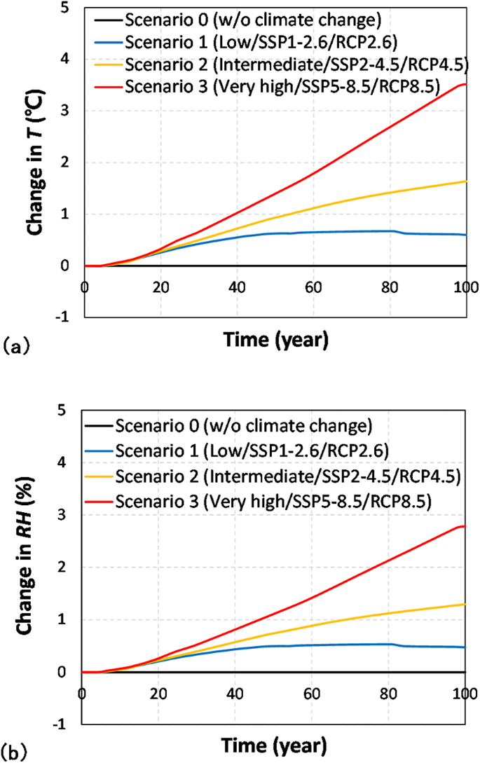
Change in the future environmental variable. (a) temperature. (b) relative humidity.

Maintenance strategy

Throughout the use stage, the maintenance strategies for the bridge were broadly categorized into preventive maintenance (PM), such as patching and repainting, and essential maintenance (EM), such as girder replacement and reconstruction46. The demands for maintenance action according to environmental conditions and climate change scenarios were estimated based on the risk assessment results. Since the PM interval (\(\:{t}_{m}\)) may vary depending on the rules or budgets of the bridge operators, LCA was performed by changing \(\:{t}_{m}\) to 5, 10, and 15 for the parameter study. EM of girder replacement was set to occur when the failure probability (\(\:{P}_{f}\)) reached the target failure probability (\(\:{P}_{f,target}\)) of 0.6% according to AASHTO MBE47. The corrosion rate can be initialized by PM, and the corrosion damage is initialized by EM. By performing risk assessment while changing the climate change scenario and \(\:{t}_{m}\), the number of PM and EM occurrences in the use stage was calculated probabilistically. This increase in the number of maintenance cycles directly led to an increase in environmental impact and cost.