Statistical and data visualization techniques to study the role of one-electron in the energy of neutral and charged clusters of Na39

Calculation method

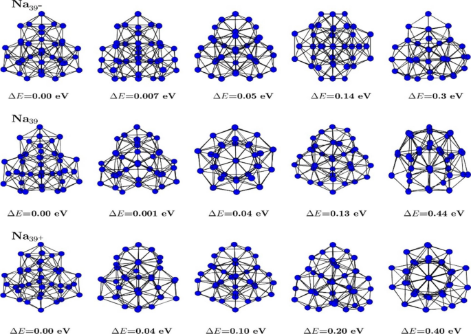
In this study, we utilize previously obtained energies and structures as inputs for our analysis. To explain how the equilibrium structures and thermodynamic data were obtained, a brief overview is provided here, with more detailed information available in Ref. 7. In Ref. 7, we employed the ab initio density functional method 35 using Vanderbilt’s ultrasoft pseudopotentials 36 within the local density approximation 37,38 as implemented in the VASP package 39. Equilibrium structures for the clusters \({Na}_{39}\), \({{Na}^{+}}_{39}\), and \({{Na}^{-}}_{39}\) were obtained to investigate the evolutionary patterns of their geometries. Approximately 200 different isomers were generated in each case, with the initial configurations derived from various ab initio constant-temperature runs at temperatures near the clusters’ melting point and beyond. For computing thermodynamic properties, the BOMD calculations were carried out at least for 10–12 different temperatures using the Nośe–Hoover thermostat 40, in the range of 120 ≤ T ≤ 400 K. Trajectory data were collected for a minimum of 240 ps, with the initial 30 ps discarded to account for thermalization.

Statistical and data visualization techniques

In this study, the statistical software R version 4.3.3 was used to perform regression analysis, fuzzy clustering analysis, and time series analysis.

Multiple linear regression analysis with dummy variable

Various statistical methods are available to analyze the impacts of one or more input variables on a response variable. Multiple linear regression is one of those methods suitable for examining the impact of quantitative inputs \({X}_{1}, \dots , {X}_{k}\) on a quantitative output \(Y\) 41, as represented by the following equation:

where \(Y\) is the output (response) variable, \({X}_{1}, \dots , {X}_{k}\) are input variables, \({\beta }_{0}\), …, \({\beta }_{k}\) are the coefficients or parameters of the model, and \(\varepsilon \) is the error term.

Using a dataset, the Eq. (1) can be estimated by:

where \({\widehat{\beta }}_{0}\) is the constant of the model, \({\widehat{\beta }}_{i}\) estimates the effect of \({X}_{i}\), and \(\widehat{Y}\) is the predicted value of \(Y\).

When facing the effects of several quantitative inputs \({X}_{1}, \dots , {X}_{k}\) and a qualitative (categorical) input \(Z\) on a quantitative output \(Y\), the multiple linear regression analysis with dummy (indicator) variables is employed. Assume that the categorical variable \(Z\) has m levels. Then, we should define m-1 dummy variables \({Z}_{1}, \dots , {Z}_{m-1}\) as follows:

The general and estimated equations of the model are respectively presented by:

and

where \({\widehat{\gamma }}_{i},i=1,\dots ,m-1,\) besides \({\widehat{\beta }}_{0}\) determine the constant of the model for the levels of Z, and \({\widehat{\delta }}_{ij}, i=1,\dots ,k,j=1,\dots ,m-1\), besides \({\widehat{\beta }}_{i}\) determine the effects of \({X}_{1}, \dots , {X}_{k}\) in different levels of Z.

Fuzzy clustering

Clustering is a useful multivariate statistical technique to categorize features or observations using 42. In applications, soft clustering approaches 43,44 work better than the traditional hard clustering approaches 45,46.

In soft clustering, especially fuzzy clustering, any point (feature or observation) can be a member of each cluster with a membership probability. It should be noticed that for each specified point, the sum of membership probabilities of the point to all clusters is equal to one. The most famous soft clustering approach is the fuzzy c-means (FCM) clustering algorithm 47.

Assume that the set \(S\) includes \(N\) records \({\overrightarrow{{\varvec{x}}}}_{k}=\left({x}_{k1},{x}_{k2},\dots ,{x}_{kD}\right), k=1,\dots , N,\) from a \(D\)-variate problem. Let \({\overrightarrow{{\varvec{c}}}}_{i}=({c}_{i1},{c}_{i2},\dots ,{c}_{iD})\) as the centroids and \({\varvec{u}}\) as the membership matrix. The soft clustering algorithm tries to divide \(S\) into \(k\) partitions \(\{{S}_{1},{S}_{2},\dots ,{S}_{k}\}\), such that:

To achieve the optimal centers and membership matrix, the error function \(SSE\) given by

is minimized subject to the constraints \(\sum_{j=1}^{k}{u}_{jx}=1\). In other words, it tries to minimize the following equation:

For a fixed membership matrix \({\varvec{u}}\), the \({c}_{ji}\) can be optimum by:

The optimal \({c}_{ji}\) is calculated by:

For a fixed cluster center matrix \({\varvec{c}}\), the \({u}_{jx}\) can be optimum by:

Equation (11) presents \(\frac{\partial E}{\partial {\alpha }_{x}}=0\).

Then, we have the following equations:

and

Autoregressive Fractionally Integrated Moving Average (ARFIMA) Time Series
9

The time series \({X}_{t}\) is said to be weakly stationary, if for all integer values of s, t, and h, the mean function of \({X}_{t}\), given by \(m\left(t\right)=E\left({X}_{t}\right),\) and the auto-covariance function of \({X}_{t},\) given by \(Cov\left({X}_{s} , {X}_{t}\right),\) are invariant, i.e.,

and

Autoregressive moving average (ARMA)

One of significant subset of stationary processes are autoregressive moving average (ARMA) time series. The ARMA processes with orders p and q (ARMA (p, q)) are presented by:

where

where \({Z}_{t}\) is a white noise process and \(B\) denotes the backward shift operator (\({B}^{j}{X}_{t}={X}_{t-j}).\) When the time series \({X}_{t}\) has a trend, the ARMA time series is inappropriate. Therefore, the autoregressive integrated moving average (ARIMA) processes can be used. The ARIMA time series of orders p, d, and q (ARIMA (p, d, q)) can be formulated by:

where \(d\) denotes the order of trend that is a natural number. The process \({(1-B)}^{d}{X}_{t}\) is a weakly stationary process. To generalize the ARIMA processes, the autoregressive fractionally integrated moving average (ARFIMA) time series are considered. For these processes, the parameter \(d\) is taken on the fractional values \(-0.5