In this section, we present a general approach to characterize EPs for open systems subject to non-Markovian noise, as illustrated in Fig. 1. To begin with, we consider an open quantum system (S) coupled to a bosonic environment (E), where the total Hamiltonian is expressed by
$${H}_{{{{\rm{tot}}}}}= {H}_{{{{\rm{S}}}}}+{H}_{{{{\rm{E}}}}}+{H}_{{{\rm{S}}}{{\rm{E}}}} \, \, {{\rm{with}}} \, \, {H}_{{{{\rm{E}}}}}={\sum}_{k}{\omega }_{k}{b}_{k}^{{{\dagger}} }{b}_{k},\\ {H}_{{{\rm{S}}}{{\rm{E}}}}= QX,\,\,{{\rm{and}}}\,X={\sum}_{k}{g}_{k}\left({b}_{k}^{{{\dagger}} }+{b}_{k}\right).$$
(2)
Here, HS and HE represent the free Hamiltonians of the system and its environment, while HSE describes their interactions. Also, ωk and gk correspond to the frequency and the coupling strength for the environmental mode bk, respectively, and Q represents an arbitrary operator acting on the system that characterizes the system-environment coupling. We consider that the environment is initialized in a Gibbs state at temperature T: \({\rho }_{{{{\rm{E}}}}}=\exp (-\beta {H}_{{{{\rm{E}}}}})/{{{\rm{tr}}}}[\exp (-\beta {H}_{{{{\rm{E}}}}})]\), where \(\beta={({k}_{{{{\rm{B}}}}}T)}^{-1}\) with kB denoting the Boltzmann constant. In this case, the exact dynamics of the open system’s reduced density matrix (within the interaction picture) can be written as
$${\rho }_{{{{\rm{S}}}}}(t)=\hat{{{{\mathcal{T}}}}}\exp \left\{\hat{{{{\mathcal{F}}}}}\left[Q,C(t)\right]\right\}{\rho }_{{{{\rm{S}}}}}(0).$$
(3)
Here, \(\hat{{{{\mathcal{T}}}}}\) denotes the time-ordering operator and \(\hat{{{{\mathcal{F}}}}}\) represents the Feynman-Vernon influence functional31, which can be expressed by
$$\hat{{{{\mathcal{F}}}}}=-\int_{0}^{t}d{t}_{1}\int_{0}^{{t}_{1}}d{t}_{2}\,Q{({t}_{1})}^{\times }\left[{C}_{{\mathbb{R}}}({t}_{1}-{t}_{2})Q{({t}_{2})}^{\times }+i{C}_{{\mathbb{I}}}({t}_{1}-{t}_{2})Q{({t}_{2})}^{\circ }\right],$$
(4)
where \(Q(t)=\exp (i{H}_{{{{\rm{S}}}}}t)Q\exp (-i{H}_{{{{\rm{S}}}}}t)\), and the superoperator notations Q(t)× = [Q(t), \(\bullet\)] and Q(t)° = {Q(t), \(\bullet\)} denote the commutator and anti-commutator, respectively. In addition, \({C}_{{\mathbb{R}}({\mathbb{I}})}\) denotes the real (imaginary) part of the environmental correlation function
$$C(t)={{{\rm{tr}}}}\left[X(t)X(0){\rho }_{{{{\rm{E}}}}}\right],$$
(5)
with \(X(t)=\exp (i{H}_{{{{\rm{E}}}}}t)X\exp (-i{H}_{{{{\rm{E}}}}}t)\). An essential feature of \(\hat{{{{\mathcal{F}}}}}\) is its exclusive dependence on the system-environment coupling operator Q and the environmental correlation function C(t). The latter can be expressed by
$$C(t)=\int_{0}^{\infty }d\omega \,\frac{J(\omega )}{\pi }\left[\coth \left(\frac{\beta \omega }{2}\right)\cos (\omega t)-i\sin (\omega t)\right],$$
(6)
where J(ω) = ∑k∣gk∣2δ(ω − ωk) represents the coupling spectral density. This property enables the reproduction of the exact open system dynamics through an auxiliary model involving a small set of fictitious damping modes, i.e., the PMs, provided that the correlation function for the artificial model aligns with Eq. (6).

a Generic system-environment model where the structured environment is captured by the spectral density function J(ω). For a given spectral density function and the corresponding environmental correlation function, the exact non-Markovian dynamics can either be described by b the PMEOM or c the HEOM with the corresponding extended Liouvillian superoperators: \({{{{\mathcal{L}}}}}_{{{\rm{S}}}+{{\rm{PM}}}}\) and \({{{{\mathcal{L}}}}}_{{{\rm{S}}}+{{\rm{ADO}}}}\). d The non-Markovian EPs can then be identified by observing the complex spectrum {λi} of these extended Liouvillian superoperators.
For a broad range of cases, the correlation function can be efficiently expressed as a finite weighted summation of exponential terms, i.e.,
$$C(t)={\sum}_{i}{\alpha }_{i}^{2}\exp (-i{\Omega }_{i}t-{\gamma }_{i}| t| /2).$$
(7)
This expression can be obtained by several approaches. For commonly used spectral densities, such as the Drude-Lorentz and Brownian motion types, analytical expressions for C(t) are available as an infinite sum of decaying exponentials (i.e., the Matsubara modes)54. In practice, this sum is truncated to balance accuracy with computational cost. More recently, the adaptive Antoulas-Anderson (AAA) algorithm64, a numerical subroutine, has been employed to optimize the underlying pole structure for the integration in Eq. (6), allowing for an efficient approximation of C(t) with a finite sum of exponentials65.
With this expression, one can construct the PMEOM:
$$ \frac{d}{dt}{\rho }_{{{\rm{S}}}+{{\rm{PM}}}}(t)={{{{\mathcal{L}}}}}_{{{\rm{S}}}+{{\rm{PM}}}}[{\, \rho }_{{{\rm{S}}}+{{\rm{PM}}}}(t)] \hfill\\ =-i[{H}_{{{\rm{S}}}+{{\rm{PM}}}},{\rho }_{{{\rm{S}}}+{{\rm{PM}}}}(t)]+{\sum}_{i}{\gamma }_{i}{{{{\mathcal{L}}}}}_{{a}_{i}}[{\, \rho }_{{{\rm{S}}}+{{\rm{PM}}}}(t)],\\ \, {{\rm{with}}} \, \, {H}_{{{\rm{S}}}+{{\rm{PM}}}}={H}_{{{{\rm{S}}}}}+{\sum}_{i}{\Omega }_{i}{a}_{i}^{{{\dagger}} }{a}_{i}+{\alpha }_{i}Q\left({a}_{i}^{{{\dagger}} }+{a}_{i}\right),$$
(8)
where, {ai} represent the PMs, and we introduce the dissipator \({{{{\mathcal{L}}}}}_{{a}_{i}}[\bullet ]={a}_{i}\,\bullet \, {a}_{i}^{{{\dagger}} }-\{{a}_{i}^{{{\dagger}} }{a}_{i},\bullet \}/2\). Notably, the environmental influences on the open system are now captured by the PMs’ frequencies Ωi, damping rates γi, and the system-PM coupling strengths αi. The exact dynamics of S can be obtained by tracing out the PMs, i.e., \({\rho }_{{{{\rm{S}}}}}(t)={{{{\rm{tr}}}}}_{{{{\rm{PM}}}}}[{\, \rho }_{{{\rm{S}}}+{{\rm{PM}}}}(t)]\), after solving the PMEOM with these PMs initialized in the thermal states.
One notable benefit of employing the PM model lies in its facilitation of establishing physical intuitions regarding the EP criteria. For instance, recent works have suggested that EPs are closely related to critical damping points for both classical and quantum systems22. As we demonstrate below, it is feasible to pinpoint EPs by balancing the system-PM coupling strength and the PM damping, leading the system to a critical damping point.
Furthermore, a systematic procedure for characterizing non-Markovian EPs based on a standard spectral analysis can be established. The main idea is grounded in the observation that both the temporal evolution of ρS+PM(t) and ρS(t) are governed by the spectral properties of the extended Liouvillian superoperator \({{{{\mathcal{L}}}}}_{{{\rm{S}}}+{{\rm{PM}}}}\). Specifically, assuming that \({{{{\mathcal{L}}}}}_{{{\rm{S}}}+{{\rm{PM}}}}\) is diagonalizable, we consider its eigenvalues and the corresponding eigenmatrices: \({\{{\lambda }_{i},{\hat{\rho }}_{{{\rm{S}}}+{{\rm{PM}}},i}\}}_{i}\). The dynamics of ρS+PM(t) can then be expressed by
$${\rho }_{{{\rm{S}}}+{{\rm{PM}}}}(t)={\sum}_{i}{c}_{i}\exp ({\lambda }_{i}t){\hat{\rho }}_{{{\rm{S}}}+{{\rm{PM}}},i}.$$
(9)
By tracing out these PMs, one can observe that the exact dynamics of the system’s reduced state follows a similar expression, replacing these eigenmatrices \({\hat{\rho }}_{{{\rm{S}}}+{{\rm{PM}}},i}\) with the reduced eigenmatrices \({\hat{\rho }}_{{{\rm{S}}},i}={{{{\rm{tr}}}}}_{{{{\rm{PM}}}}}({\hat{\rho }}_{{{\rm{S}}}+{{\rm{PM}}},i})\), namely,
$${\rho }_{{{{\rm{S}}}}}(t)={\sum}_{i}{c}_{i}\exp ({\lambda }_{i}t){\hat{\rho }}_{{{\rm{S}}},i}.$$
(10)
To describe EPs, one considers a family of parametrized extended Liouvillian superoperators \({{{{\mathcal{L}}}}}_{{{\rm{S}}}+{{\rm{PM}}}}({{{\boldsymbol{\xi }}}})\), bearing in mind that ξ includes the parameters related to both the system and the structured environments. Since \({{{{\mathcal{L}}}}}_{{{\rm{S}}}+{{\rm{PM}}}}({{{\boldsymbol{\xi }}}})\) is generally non-Hermitian, EPs could potentially exist in the parameter space. For instance, let ξEPn represent an nth-order EP in the parameter space, where n different eigenvalues and the corresponding eigenmatrices \({\{{\lambda }_{i},{\hat{\rho }}_{{{\rm{S}}}+{{\rm{PM}}},i}\}}_{i\in A}\) coalesce into \(\{{\lambda }_{{{{\rm{EP}}}}},{\hat{\rho }}_{{{\rm{S}}}+{{\rm{PM}}},{\lambda }_{{{{\rm{EP}}}}}}\}\). Here, A denotes a set of indices. Due to the coalescence of the eigenmatrices, the corresponding n-dimensional eigensubspace for \({{{{\mathcal{L}}}}}_{{{\rm{S}}}+{{\rm{PM}}}}({{{{\boldsymbol{\xi }}}}}_{{{{\rm{EP}}}}})\) cannot be diagonalized. Nevertheless, a Jordan block for the subspace can be constructed by introducing generalized eigenmatrices \({\{{\hat{\rho }}_{{{\rm{S}}}+{{\rm{PM}}},{\lambda }_{{{{\rm{EP}}}}}}^{( \, \, j)}\!\}}_{j=0,\cdots,n-1}\), such that the system dynamics can be expressed by
$${\rho }_{{{{\rm{S}}}}}(t)={\sum}_{i\notin A}{c}_{i}{e}^{{ \, \lambda }_{i}t}{\hat{\rho }}_{{{\rm{S}}},i}+{e}^{{\, \lambda }_{{{{\rm{EP}}}}}t}{\sum}_{j=0}^{n-1}{\sum}_{m=0}^{j}\frac{{t}^{m}{\tilde{c}}_{m}}{m!}{\hat{\rho }}_{\,{{\rm{S}}},{\lambda }_{{{{\rm{EP}}}}}}^{(\, \, j)},$$
(11)
where the reduced generalized eigenmatrices are introduced as
$${\hat{\rho }}_{\,{{\rm{S}}},{\lambda }_{{{{\rm{EP}}}}}}^{(\, \, j)}={{{{\rm{tr}}}}}_{{{{\rm{PM}}}}}\left({\hat{\rho }}_{\,{{\rm{S}}}+{{\rm{PM}}},{\lambda }_{{{{\rm{EP}}}}}}^{(\, \, j)}\right).$$
(12)
Equation (11) suggests that the polynomial time dependence, a common dynamical signature of EPs, could be observed in the reduced dynamics of the open system. In essence, the PMEOM provides an intuitive and direct route to investigate EPs beyond the BMS approximation, and this approach is compatible with the conventional spectral analysis by introducing the (generalized) reduced eigenmatrices.
It is worth noting that an alternative approach is to consider the framework of the HEOM. In this context, a set of ADOs is introduced to capture the non-Markovian and non-perturbative effects54,56,58,66,67,68. Similarly, we can define the extended quantum state ρS+ADO that contains both the system-reduced state and the ADOs. The dynamics of the extended state are governed by the extended Liouvillian superoperator \({{{{\mathcal{L}}}}}_{{{\rm{S}}}+{{\rm{ADO}}}}\). The system’s reduced state can be obtained through a linear operation, specifically \({\rho }_{{{{\rm{S}}}}}(t)={{{\mathcal{P}}}}[{\rho }_{{{\rm{S}}}+{{\rm{ADO}}}}(t)]\), where \({{{\mathcal{P}}}}\) is a superoperator for discarding all the ADOs (see Methods). Therefore, the EPs for non-Markovian open quantum systems can also be equivalently characterized under the framework of the HEOM by introducing the corresponding (generalized) reduced eigenmatrices, which are expressed as \({\tilde{\rho }}_{{{\rm{S}}},i}={{{\mathcal{P}}}}({\, \tilde{\rho }}_{{{\rm{S}}}+{{\rm{ADO}}},i})\) and \({\tilde{\rho }}_{\,{{\rm{S}}},{\lambda }_{{{{\rm{EP}}}}}}^{(\, \, j)}={{{\mathcal{P}}}}({\, \tilde{\rho }}_{\,{{\rm{S}}}+{{\rm{ADO}}},{\lambda }_{{{{\rm{EP}}}}}}^{(\, \, j)})\).
Spin-boson model
To gain a more intuitive understanding, we apply the PMEOM to the prototype spin-boson model, showing that additional EPs without Markovian analog can be observed by adjusting the structural characteristics of the environment’s spectral density. To simplify our analysis, we consider a zero-temperature environment and adopt the rotating-wave approximation (RWA), where the system-environment interaction in Eq. (2) and the system-PM coupling in Eq. (8) can be expressed by \({\sum} _{k}{g}_{k}(\tilde{Q}{b}_{k}^{{{\dagger}} }+{\tilde{Q}}^{{{\dagger}} }{b}_{k})\) and \({\sum }_{i}{\alpha }_{i}(\tilde{Q}{a}_{i}^{{{\dagger}} }+{\tilde{Q}}^{{{\dagger}} }{a}_{i})\), respectively. Furthermore, we consider a scenario where the spectral density function J(ω) is well localized in the vicinity of a high-frequency \(\omega_0\) ≫ 0, enabling us to effectively approximate the correlation in Eq. (6) by extending the lower limit of the integral to negative infinity. Note that the assumptions mentioned above are also considered in the original proposals of PMEOM38,39,40.
The model involves a qubit representing the open system, where the system Hamiltonian and system-environment coupling operator are \({H}_{{{{\rm{S}}}}}={\omega }_{0}\left\vert e\right\rangle \left\langle e\right\vert\) and \(\tilde{Q}={\sigma }_{-}\), respectively. Such an interaction can lead to an energy exchange between the qubit and the environment, therby inducing non-Hermiticity for the system. Here, \(\omega_0\) denotes the qubit transition frequency between the ground state \(\left\vert g\right\rangle\) and the excited state \(\left\vert e\right\rangle\), and \({\sigma }_{+}=\left\vert e\right\rangle \left\langle g\right\vert\) (\({\sigma }_{-}=\left\vert g\right\rangle \left\langle e\right\vert\)) represents the raising (lowering) operator. We consider a Lorentzian spectral density that is expressed by
$${J}_{L}(\omega )=\frac{1}{2}\frac{\varGamma {\varLambda }^{2}}{{(\omega -{\omega }_{0})}^{2}+{\varLambda }^{2}},$$
(13)
where Γ and Λ denote the coupling strength and the spectral width, respectively. In the interaction picture and under the earlier specified assumption of extending the spectral density function to negative frequencies, the environmental correlation function can be expressed by a single exponential term, i.e., \(C(t)=(\varGamma \varLambda /2)\exp (-\varLambda | t| )\). Therefore, the PMEOM can be constructed by introducing a single PM with the damping rate γ = 2Λ and the qubit-PM coupling strength \(\alpha=\sqrt{\varGamma \varLambda /2}\). As aforementioned, the PM representation provides a physical intuition that the EP could be located by balancing γ and α (or Γ and Λ) so that the system reaches a critical damping point.
The corresponding extended Liouvillian superpoerator \({{{{\mathcal{L}}}}}_{{{\rm{S}}}+{{\rm{PM}}}}(\varGamma,\varLambda )\) can be described by a 9 × 9 non-Hermitian matrix in the single-excitation subspace (Supplementary Information). The spectrum is illustrated in Fig. 2, revealing that Γ = Λ/2 corresponds to a second-order EP (EP2) and a third-order EP (EP3). Notably, these EPs are unobservable in the Markovian wide-band limit. Specifically, in such a limit, the spectral width (and thus the damping rate of the PM) becomes infinite, Λ → ∞. Therefore, the PM can be adiabatically eliminated, and the dynamics are governed by a qubit-only Markovian master equation, i.e., \({\dot{\rho }}_{{{{\rm{S}}}}}(t)=\varGamma [2{\sigma }_{-}{\rho }_{{{{\rm{S}}}}}(t){\sigma }_{+}-\{{\sigma }_{+}{\sigma }_{-},{\rho }_{{{{\rm{S}}}}}(t)\}]/2\). Intuitively, there is only one qubit decay channel without internal tunneling between the qubit energy levels, thereby EP does not emerge in this scenario17.
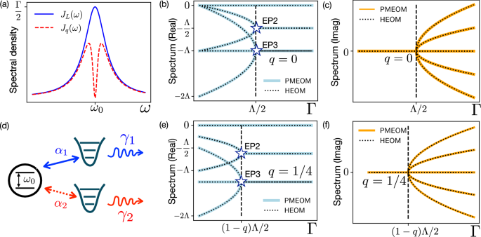
a Lorentzian JL(ω) and band gap Jq(ω) spectral densities centered at the qubit transition frequency \(\omega_0\). d The effects of these spectral densities can be represented by two PMs: The Lorentzian spectral density can be described by the upper PM with qubit-PM coupling strength \({\alpha }_{1}=\sqrt{\varGamma \varLambda /2}\) and PM’s damping rate γ1 = 2Λ, while the band gap is characterized by the lower PM with the non-Hermitian coupling \({\alpha }_{2}=i\sqrt{q\varGamma \varLambda /2}\) and damping rate γ2 = 2qΛ, where the red dashed line signifies the unphysical nature of this PM. b, c The real and imaginary parts of the spectrum of the extended Liouvillian for the gapless scenario (q = 0). Two EPs, EP2 and an EP3 emerge at the coupling strength Γ = Λ/2. e, f The real and imaginary parts of the spectrum of the extended Liouvillian with q = 1/4. The EP criterion becomes Γ = (1 − q)Λ/2. The dotted curves in b, c, e, f represent the spectrum of the extended superoperators for HEOM (see Supplementary Information for detailed derivations).
Let us proceed with a deeper analysis of the EP dynamical signatures. According to Fig. 2b, c, the EP condition pinpoints a real-to-complex transition in the spectrum. In other words, the EP condition corresponds to a critical damping point, separating the overdamped (pure decay) and underdamped (oscillatory) regimes. By investigating the generalized eigenmatrices for the extended superoperator at the EP condition, i.e., \({{{{\mathcal{L}}}}}_{{{\rm{S}}}+{{\rm{PM}}}}(\varGamma=\varLambda /2)\), we conclude that the qubit coherence and population dynamics are respectively determined by the EP2 and EP3, resulting in observing first-order and second-order polynomial time dependencies:
$$\left\langle e\right\vert {\rho }_{{{{\rm{S}}}}}(t)\left\vert g\right\rangle = \frac{1}{2}(\varLambda t+2){e}^{-\frac{1}{2}\varLambda t}\left\langle e\right\vert {\rho }_{{{{\rm{S}}}}}(0)\left\vert g\right\rangle,\hfill\\ \left\langle e\right\vert {\rho }_{{{{\rm{S}}}}}(t)\left\vert e\right\rangle = \frac{1}{4}\left({\varLambda }^{2}{t}^{2}+4\varLambda t+4\right){e}^{-\varLambda t}\left\langle e\right\vert {\rho }_{{{{\rm{S}}}}}(0)\left\vert e\right\rangle .$$
(14)
Furthermore, the transition from the overdamped to underdamped regimes opens up the possibility of observing enhanced sensitivity to external perturbations in the vicinity of the EP. For instance, consider a small perturbation in the coupling strength, represented as Γ → Λ(1 + ϵ)/2, with ϵ > 0. This perturbation induces splittings in the imaginary parts of the eigenvalues, resulting in oscillatory dynamics. Notably, these splittings scale as \(\sqrt{\epsilon }\), indicating the sensitivity enhancement in the characteristic frequency of the oscillatory behavior. For this model, both the qubit excited state population and coherence vanish periodically. We choose, for simplicity, the first vanishing time tvanish of the qubit coherence to capture the system’s oscillations. One can find \({t}_{\,{{\rm{vanish}}}\,}^{-1}\approx \varLambda \sqrt{\epsilon }/2+O\left(\epsilon \right)\), which implies that tvanish is sensitive to external perturbation when the system is prepared at the EP.
Up to this point, we only tune the environmental parameters without changing the shape of the Lorentzian profile, and we have shown that such an adjustment does not modify the structure of the PMEOM. Let us further consider a more complex scenario, where an additional parameter can drastically modify the spectral shape. To this end, we introduce a band-gap structure to the Lorentzian background31, which is modeled as
$${J}_{q}(\omega )={J}_{L}(\omega )-\frac{1}{2}\frac{\varGamma {(q\varLambda )}^{2}}{{(\omega -{\omega }_{0})}^{2}+{(q\varLambda )}^{2}},$$
(15)
where the band gap is located at the frequency \(\omega_0\), such that Jq(\(\omega_0\)) = 031 [see also Fig. 2a], and the parameter q ∈ (0, 1] is used to control the relative width for the band gap. The environmental correlation function is now expressed by two exponential terms:
$$C(t)=\frac{\varLambda \varGamma }{2}\exp (-\varLambda | t| )-\frac{q\varLambda \varGamma }{2}\exp (-q\varLambda | t| ).$$
(16)
Accordingly, the PMEOM for the exact dynamics involves two PMs (a1 and a2), each characterized by the qubit-PM coupling strengths and PM damping rates [see also Fig. 2d]: \(\left\{{\alpha }_{1}=\sqrt{\varGamma \varLambda /2},{\alpha }_{2}=i\sqrt{q}{\alpha }_{1},{\gamma }_{1}=2\varLambda,{\gamma }_{2}=q{\gamma }_{1}\right\}.\) The spectrum of the corresponding extended Liouvillian superoperator is presented in Fig. 2e, f, suggesting that the EP criterion becomes
$$\varGamma=(1-q)\varLambda /2.$$
(17)
Consequently, including a band gap into the environmental spectral profile leads to a displacement of the EP in the parameter space. In this case, the system requires a smaller coupling strength to reach the EP criterion compared to the case of the previous gapless Lorentzian environment.
We remark that α2 is purely imaginary, so it does not directly correspond to a physical mode. This characteristic causes the HS+PM to become non-Hermitian43. Nevertheless, the reduced dynamics of the qubit is still exact and well-behaved as long as the PMEOM is consistent with the given C(t)43. Furthermore, in Fig. 2 and Supplementary Information, we demonstrate that the spectrum of the extended Liouvillian operators for the HEOM is consistent with that of PMEOM.
Another notable aspect is that the EP condition also aligns with the onset of non-Markovianity by utilizing the Breuer–Laine–Piilo (BLP)69 and the Rivas–Huelga–Plenio (RHP)70 non-Markovianity measures. Specifically, for the spin-boson model, the analytical solution for the qubit-reduced state is expressed as31
$$\left\langle e\right\vert {\rho }_{{{{\rm{S}}}}}(t)\left\vert e\right\rangle =\left\langle e\right\vert {\rho }_{{{{\rm{S}}}}}(0)\left\vert e\right\rangle | G(t){| }^{2},\\ \left\langle g\right\vert {\rho }_{{{{\rm{S}}}}}(t)\left\vert e\right\rangle =\left\langle g\right\vert {\rho }_{{{{\rm{S}}}}}(0)\left\vert e\right\rangle G(t).$$
(18)
Here, G(t) is commonly referred to as the decoherence function71, which is given by
$$G(t)=\frac{\varGamma {e}^{-\varLambda {\delta }_{+}t/2}}{2q\varLambda -\varGamma {\delta }_{-}}\left[\frac{{\delta }_{+}\sqrt{\varLambda {\delta }_{-}}\sinh \left(\eta t\right)}{\sqrt{2\varGamma+\varLambda {\delta }_{-}}}-{\delta }_{-}\cosh \left(\eta t\right)\right]+\frac{2q\varLambda }{2q\varLambda -\varGamma {\delta }_{-}}.$$
(19)
with δ± = q ± 1 and \(\eta=\sqrt{\varLambda {\delta }_{-}(2\varGamma+\varLambda {\delta }_{-})}/2\). It is well-established that for both the BLP and the RHP measures, the transition from Markovian to non-Markovian dynamics occurs when ∣G(t)∣ shifts from pure decay to oscillatory behavior71. Consequently, the transition point can be identified from Eq. (18) as δ−Λ = −2Γ, or equivalently Γ = (1 − q)Λ/2, precisely aligning with the EP condition in Eq. (17). In Fig. 3, we present the dynamics of the decoherence function ∣G(t)∣ for different values of Γ, where ΓEP = (1 − q)Λ/2 corresponds to the EP criterion. One can observe that the dynamics changes from monotonic decay (overdamped) to oscillatory behavior (underdamped), as Γ increases and crosses the EP at Γ = ΓEP.
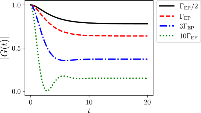
Here, ΓEP = (1 − q)Λ/2, and we set Λ = 1 and q = 1/4.
Linear bosonic systems with adjoint pseudomode-equation of motion
The PMEOM in Eq. (8) offers significant flexibility by allowing both the system Hamiltonian HS and the coupling operator Q to be arbitrary. This utility facilitates the extension of our analysis to a variety of open quantum systems. As an illustrative application, we now explore linear bosonic systems, which have garnered significant interest in the study of both LEPs and HEPs11,18,20,21,24. Specifically, we examine a general Hamiltonian with M coupled modes, expressed as
$${H}_{{{{\rm{S}}}}}={\sum}_{k=1}^{M}{\Omega }_{k}{c}_{k}^{{{\dagger}} }{c}_{k}+{\sum}_{j
(20)
where Ωk denotes the frequency associated with the mode ck, and χj,k represents the coherent coupling between the modes j and k.
In the Heisenberg picture, the dynamics are governed by the following adjoint PMEOM:
$$ \frac{d}{dt}{O}_{{{\rm{S}}}+{{\rm{PM}}}}(t)=i[{H}_{{{\rm{S}}}+{{\rm{PM}}}},{O}_{{{\rm{S}}}+{{\rm{PM}}}}(t)]\hfill\\ +{\sum}_{i}\frac{{\gamma }_{i}}{2}\left(2{a}_{i}^{{{\dagger}} }{O}_{{{\rm{S}}}+{{\rm{PM}}}}(t){a}_{i}-\left\{{a}_{i}^{{{\dagger}} }{a}_{i},{O}_{{{\rm{S}}}+{{\rm{PM}}}}(t)\right\}\right),$$
(21)
where OS+PM(t) denotes an arbitrary operator acting on the joint system, S + PM. To facilitate the analysis, we define a vector containing the annihilation operators for both the system modes and the PMs:
$${{{\bf{v}}}}={\left({c}_{1},\cdots,{c}_{M},{a}_{1},\cdots,{a}_{i},\cdots \right)}^{T}.$$
(22)
Focusing on the amplitudes of these modes, we denote
$$\begin{array}{l}\left\langle{{{\bf{v(t)}}}}\right\rangle={(\left\langle{c}_{1}(t)\right\rangle,\cdots,\left\langle{c}_{M}(t)\right\rangle,\left\langle{a}_{1}(t)\right\rangle,\cdots,\left\langle{a}_{i}(t)\right\rangle,\cdots)}^{T},\\ \,{{\rm{with}}}\,\left\langle a(t)\right\rangle={{{\rm{tr}}}}[a(t){\rho}_{{{\rm{S}}}+{{\rm{PM}}}}(0)].\end{array}$$
(23)
Through the adjoint PMEOM, the dynamics for the amplitudes are determined by the effective NHH
$${H}_{{{\rm{eff}}},{{\rm{S}}}+{{\rm{PM}}}}={H}_{{{\rm{S}}}+{{\rm{PM}}}}-i{\sum}_{i}{\gamma }_{i}{a}_{i}^{{{\dagger}} }{a}_{i}/2={{{{\bf{v}}}}}^{{{\dagger}} }{{{{\bf{H}}}}}_{{{\rm{eff}}},{{\rm{S}}}+{{\rm{PM}}}}{{{\bf{v}}}},$$
(24)
where Heff,S+PM is a matrix representation of the NHH. Specifically, one obtains
$$\left\langle \dot{{{{\bf{v}}}}}(t)\right\rangle=i{{{{\bf{H}}}}}_{{{\rm{eff}}},{{\rm{S}}}+{{\rm{PM}}}}\left\langle {{{\bf{v}}}}(t)\right\rangle,$$
(25)
indicating that potential EPs can now be encoded in Heff,S+PM.
For a concrete example, we examine a two-mode system with
$${\chi }_{1,2}=\chi \, \, {{\rm{and}}}\, \, {\Omega }_{1}={\Omega }_{2}={\omega }_{0}.$$
(26)
Also, we consider one of the modes (c2) is further coupled to a Lorentzian environment in zero temperature, as described in Eq. (13). In the wide-band limit (Λ → ∞), the resulting system-only effective non-Hermitian Hamiltonian within the rotating frame is given by:
$${{{{\bf{H}}}}}_{{{\rm{eff}}},{{\rm{S}}}}=\left(\begin{array}{cc}0&\chi \\ \chi &i\frac{\varGamma }{2}\end{array}\right).$$
(27)
The corresponding eigenvalues are \((i\varGamma \pm \sqrt{16{\chi }^{2}-{\varGamma }^{2}})/4\), indicating the presence of an EP2 if ∣χ∣ = Γ/4, with the degenerate eigenvalue iΓ/4. The dynamics at the EP2 can be derived as:
$$\left\langle {c}_{1}(t)\right\rangle ={e}^{-\varGamma t/4}\left[\left\langle {c}_{1}(0)\right\rangle+\frac{\varGamma t}{4}\left(\left\langle {c}_{1}(0)\right\rangle+i\left\langle {c}_{2}(0)\right\rangle \right)\right]\\ \left\langle {c}_{2}(t)\right\rangle =\frac{1}{4}{e}^{-\varGamma t/4}\left[i\left\langle {c}_{1}(0)\right\rangle \varGamma t+\left\langle {c}_{2}(0)\right\rangle (4-\varGamma t)\right].$$
(28)
As expected, the first-order time dependence is observed due to the EP2.
With a finite width Λ, the effective Hamiltonian takes the form:
$${{{{\bf{H}}}}}_{{{\rm{eff}}},{{\rm{S}}}+{{\rm{PM}}}}=\left(\begin{array}{ccc}0&\chi &0\\ \chi &0&\sqrt{\frac{\varGamma \varLambda }{2}}\\ 0&\sqrt{\frac{\varGamma \varLambda }{2}}&i\varLambda \end{array}\right).$$
(29)
By matching the coefficients of the characteristic polynomial, an EP3 is identified with the following criteria:
$$\left\{| \chi |=\frac{\varLambda }{3\sqrt{3}},\,\varGamma=\frac{16\varLambda }{27}\right\},$$
(30)
and the degenerate eigenvalue is iΛ/3. In this case, the dynamics is written as:
$$\left\langle {c}_{1}(t)\right\rangle= \frac{{e}^{-\varLambda t/3}}{27}\bigg[\left\langle {c}_{1}(0)\right\rangle \left({\varLambda }^{2}{t}^{2}+9\varLambda t+27\right)\\ +\left\langle {c}_{2}(0)\right\rangle i\sqrt{3}\varLambda t(\varLambda t+3)\bigg],\hfill\\ \left\langle {c}_{2}(t)\right\rangle= \frac{{e}^{-\varLambda t/3}}{9\sqrt{3}}\bigg[\left\langle {c}_{1}(0)\right\rangle i\varLambda t(\varLambda t+3)\hfill\\ -\left\langle {c}_{2}(0)\right\rangle \sqrt{3}\left({\varLambda }^{2}{t}^{2}-3\varLambda t-9\right)\bigg],$$
(31)
where the second-order time dependence can be observed due to the EP3.
In Fig. 4, we present the real part of the eigenvalues for different values of χ and Λ. The EP2 (yellow dashed curve) originates from the prediction in the wide-band limit [i.e., Eq. (27)]. As Λ decreases, one can observe that the EP2 is transformed into the EP3 (white dashed curve) when Λ becomes sufficiently small. This demonstrates that the order of the EP can be upgraded by adjusting the characteristics of the structured environment.

Real part of the eigenvalues λi (i = 1, 2, 3), corresponding to the effective Hamiltonian described in Eq. (29), as a function of the spectral width Λ and coupling strength χ. Here, we set Γ = 1. The yellow and white dashed curves represent the EP2 and EP3 curves, respectively.
This upgrade can lead to a further enhancement in the system’s sensitivity. For instance, we introduce a perturbation ϵ > 0 to the coupling strength χ → χ(1 + ϵ). In the vicinity of the EP3, the eigenvalues take the form
$$\left\{i\frac{\varLambda }{3}+{x}_{1}\varLambda {\epsilon }^{\frac{1}{3}}+O\left({\epsilon }^{\frac{2}{3}}\right),i\frac{\varLambda }{3}+{x}_{2}\varLambda {\epsilon }^{\frac{1}{3}}+O\left({\epsilon }^{\frac{2}{3}}\right),\right.\left.i\frac{\varLambda }{3}+{x}_{3}\varLambda {\epsilon }^{\frac{1}{3}}+O\left({\epsilon }^{\frac{2}{3}}\right)\right\},$$
(32)
where x1, x2, and x3 are constants. We can observe a cubic-root bifurcation for the EP3 in response to the external perturbation, signifying sensitivity enhancement.
Intuitively, one may anticipate that higher-order EPs may emerge when considering an environment with a more complicated spectral structure, which requires more PMs to capture the non-Markovian dynamics and increases the dimension of the non-Markovian NHHs