In this section we describe not only the methods used in the production of population grids, but also the primary data. Beyond the methods, it is necessary to understand the initial information and its limitations to evaluate the goodness of the results obtained.
Although the main sources of information for the generation of the top-down population grids are a historical compilation of cadastre data4 and the homogenised census population data at municipal level –Local Administrative Units (LAU)–5,6, the work uses other complementary sources to improve quality and complete the results. First, we describe in detail the different databases used, taking into account their limitations in space and time, and then we detail the production methods used.
Historical settlement data compilation for Spain (1900–2020): HISDAC-ES
Uhl et al.4 download and process the cadastral information of more than 12 million buildings and their features. After a certain harmonisation of the different existing cadastres in Spain –five in total–, they transform the vector information of the building contours into point vector information, and the different features are transformed into raster layers with 100 m × 100 m resolution. The database is labelled as HISDAC-ES, and we used version 2. Validation exercises carried out by Uhl et al.3 indicate that the database is of acceptable quality, especially in recent times, probably higher than remote sensing products, although at the beginning of the century the quality of the information is considerably reduced due to the problem of dating the buildings in the cadastre, the so-called survivorship bias.
The volume of information generated is enormous –743 raster layers– and many of the variables provided have been classified by five-year intervals since 1900. The raster information is provided in different coordinate reference systems (CRS), including the European Terrestial Reference System 1989 (ETRS89) – Lambert Azimutal Equal Area (LAEA) –EPSG:3035–, which is the reference system for European grids7, for all Spanish territory.
This information constitutes the main support on which the population will be allocated. Of all the variables offered, the most appropriate for redistributing the resident population by administrative unit over the territory –grid cells with a resolution of 100 m × 100 m– is total building indoor area (RES_BIA), which is available for each decade from 1900 to 2020 –approximate in line with the decennial census–. This variable includes the two most relevant factors in the processes of spatial disaggregation of the population8: the residential function and an indicator of the height of the buildings.
However, cadastral information is not uniform in space and time, and this affects the quality of the population redistribution.
From the spatial point of view, the existence of 5 cadastres for the whole territory, one for the majority of Spain, and 4 for each of the provinces under a different tax system from the rest of the Spanish territory –the 3 provinces of the Basque Country and Navarre– affects the uniformity of the available information.
For example, RES_BIA is not available in any year for the 3 Basque provinces –Araba/Álava, Gipuzkoa and Bizkaia–. Simply this variable is not in the data model of the cadastres of the Basque Country. For Araba/Álava we only have information on residential building footprint area (RES_BUFA), so that we lose information about the height of the buildings. And for Gipuzkoa and Bizkaia we do not even have information on the use of the building, so that only the building footprint area (BUFA) is available. As a result, the disaggregation process should incorporate information from these two variables, RES_BUFA, and BUFA, in some cases, as well as taking special care with the Basque provinces.
As mentioned at the beginning of the section, if we go back in time, things get worse. As recognized by Uhl et al.4, the HISDAC-ES database has some deficiencies in its early years. This situation is not uniform in space and affects some places more than others. The main problem is the so-called survivorship bias. The HISDAC-ES database infers the age of the building from the date given in the cadastral information, but this date may not correspond to the initial date of construction of the building. The reason is that cadastre changes the date of construction of a building if there has been a restoration or modification of the building of a certain entity and does not keep record of these changes –at least in the available public information–. As a result, it remains unknown whether a construction date represents the truly first establishment of a building at a given location or whether there was a similar built-up structure existing prior to that. The problem is noted by Uhl et al.4, section 4.6, which indicate how it is especially evident for some municipalities at the beginning of the 20th century and urge users to take precautions when analysing the data in the long term. To some extent, our results reflect these limitations, since the support on which we place the population is based on Cadastre data. However, we will mitigate the so-called survivorship bias by using auxiliary information in extreme cases.
Additionally, minor issues warrant consideration. To illustrate, we may cite the case of buildings that existed in the past but have since been demolished. Such buildings are no longer included in the cadastre and, therefore, are not reflected in HISDAC-ES. Furthermore, the function of a given building within the cadastre may be its current function, although it is possible that this function may have differed in the past. Furthermore, it is unclear whether all the characteristics of a building are based on the same date of measurement or if they were recorded on the date of construction, which may differ from the date of measurement. As previously stated, HISDAC-ES is the product of the integration of five distinct cadastres, each with its own data model. Consequently, inconsistencies may exist between the data sets. Indeed, it has already been stated that certain crucial variables are not accessible in all instances. Furthermore, the treatment of buildings as point elements, rather than polygonal, and their management as raster layers, rather than with the original vector information, introduces certain distortions. Given the magnitude of the database, these distortions are necessary to reduce the computational burden. Ultimately, it is essential to consider the frequency of updates to the cadastre data, a factor that will be particularly pertinent for records from earlier periods.
In any case, all available evidence suggests that these are relatively minor issues in comparison to the survivorship bias. However, it is essential to consider them when evaluating the results and to recognise that they should diminish over time, given that they currently have a lesser impact on the available information than they did at the beginning of the 20th century.
To get an idea of the importance of the survivorship bias in extreme cases we can examine which municipalities lack cadastral information in the different census years of the twentieth century. If we intersect the municipal boundaries with the layers of RES_BIA, RES_BUFA and BUFA of HISDAC-ES, we will observe that none of the municipalities have zero intersection only from 1970. Even in 1960, there is a municipality that does not have information about buildings in HISDAC-ES. It is a small municipality, Beizama (20020) in the province of Gipuzkoa, with only 460 inhabitants. Of course, this problem gets worse as we go back in time. In 1950, this lack of information affected 4 municipalities, 15 in 1940, 29 in 1930, 57 in 1920, 111 in 1910 and 171 in 1900. In all cases, except for a minor exception in the first decades of the 20th century, these are very small municipalities.
It should be noted that this is a general problem that affects all the municipalities, although it manifests itself in an extreme way in some more than others and is also present in large cities. Natural aggregation to cells, especially 1 km × 1 km, dilutes this problem and smooths the survivorship bias, although the precise quantification of the problem is extremely difficult.
A problem related to the survivorship bias, not mentioned in Uhl et al.4, has to do with the dating of many rural isolated farmhouses whose cadastre date does not really correspond to the date of construction. Many of these buildings were inhabited at the beginning of the 20th century and gradually ceased to be so throughout the second half of that century. The indications of this incorrect dating are evident from the fieldwork and direct consultation to the cadastre data of certain buildings.
There is no apparent solution to this type of problem, but it is necessary to be aware of it to be able to evaluate the results obtained.
What is obvious is that the information of HISDAC-ES must be complemented with another, especially in the first decades of the 20th century if we start from municipal information to generate historical population grids.
Historical municipal population data: 1900–2021
The main source of population information is the homogeneous database of Goerlich et al.5,6. These authors generate estimates of municipal population with the structure of municipalities from the 2011 census, so that they consider the municipal alterations –mergers and segregations, total and partial– occurred between 1900 and 2011. They also develop a taxonomy of changes9 with the corresponding associated database6. We therefore have homogeneous municipal populations for the 8,116 municipalities that appear in the 2011 census, with their associated vector boundary mapping. In addition, to reach the most recent date, the database is expanded with the populations of the 8,131 municipalities of the 2021 census carried out by the INE10.
The contours of the municipalities come from the National Geographical Institute (IGN)11 with reference dates 01/01/2012, for the period 1900–2011 –8,116 municipalities–, and 01/01/2019, for 2021 –8,131 municipalities–. Since the IGN municipal enclosures and boundary limit lines database is continuously updated and the IGN does not maintain historical data, these are collected and organized by Goerlich and Perez12.
Settlement coordinates from 1887 census: ESPAREL
As has become clear in the description of HISDAC-ES at the beginning of this section, we must incorporate external information that mitigates, as far as possible, the survivorship bias.
An independent geocoding project of the historical population entities contained in the gazetteers of the late eighteenth and nineteenth centuries is ESPAREL13 (https://www.esparel.com/). The main objective of ESPAREL has been to generate a spatial data infrastructure (SDI) that allows linking the spatial planning of the Old Regime with that of the liberal State at the end of the 19th century, and at the same time with the current one. For this purpose, the existing population entities in the 1787 census –census of Floridablanca–, and those of the 1887 Spanish Gazetteer –corresponding to the census of the same year– have been linked with the Basic General Gazetteer of Spain (NGBE), which is geocoded, as well as other external geocoded information currently available from regional cartographic institutes or map viewers accessible through external queries from APIs.
From our point of view, what matters is that the gazetteer of 1887 is relatively close to 1900, which is our first year for the generation of historical population grids from HISDAC-ES, and for which we have the point coordinates of 58,837 population entities, covering almost all the current municipalities. We incorporate this information for those municipalities in which HISDAC-ES lacks it. This solution addresses all the aforementioned cases, with the exception of those pertaining to the four recently established municipalities. The homogeneous populations of Goerlich et al.5,6 indicate the existence of population in these municipalities, however, neither the Cadastre nor the HISDAC-ES provides geocoded data that enables the delineation of the population within these areas. These municipalities are Badia del Vallès (08904), Vegaviana (10902), Alagón del Río (10903) and Vencillón (22909), and its population only exceeds 1,000 inhabitants for Badía del Vallès (08904) in 1950. In the other years the municipalities for which we lack support to allocate the population are extremely small. For example, in 1900 these populations ranged between 276 inhabitants for Badía del Vallès (08904) and 5 inhabitants for Alagón del Río (10903). Locating the population of these municipalities in the coordinates of the municipal capital does not entail distortion in its spatial distribution.
It should be remembered that the geocoded information of ESPAREL does not refer to buildings, but to the population entity itself. However, the number of buildings and their plants are available in the database, and, by construction, they are residential buildings. From this information a variable was constructed which adds the buildings once multiplied by their plants, which in a certain way represents the closest to the variable RES_BIA of HISDAC-ES, except that the coordinates do not correspond to individual buildings, but to the population entity. This vector point information was transformed into a raster layer with the same structure as the HISDAC-ES layers. Note that each entity will belong to a single cell of 100 m × 100 m, regardless of its size, but since these are entities of low demographic weight this is not expected to generate many distortions, especially on cells added to a resolution of 1 km × 1 km.
As a last resort, for the municipalities for which we do not find information either in ESPAREL, we use the coordinate of the capital of the municipality, which is available in the Gazetteer of Municipalities and Population Entities (NGMEP) of the IGN. Like the coordinates of ESPAREL this vector point information was transformed into a raster layer with the same structure as those of HISDAC-ES, and the population of the municipality assigned to the corresponding cell. The small size of the population in this case makes distortions minimal.
In addition to the above information, used in the process of downscaling the municipal population to the grid, the data from the 2021 census grid, GEOSTAT2021, published by INE10, and the population data from the Global Human Settlement Layer (GHSL)14, version R2023A2, with resolution of 1 km × 1 km, for the years 1980, 1990, 2000, 2010 and 2020 were used for validation purposes to compare their results with those obtained by our methods. The GHSL is a worldwide product that had to be masked by Spain’s administrative boundaries for comparison with our results. All data sources are openly available.
Downscaling historical municipal population data
The methods are relatively simple and are not very different from those used in the production of the GHSL population grids15.
The approach is based on the well-known vector/raster based dasymetric mapping16,17 relying mainly on the variable RES_BIA from HISDAC-ES to restrict and refine the distribution of people in space. Even in 1900, this covers 93% of municipalities, that increases to 97% in 2021. When, for a given municipality, this information is insufficient or non-existent other, less appropriate, variables are used following a clear predefined order. Figure 1 shows the workflow of the population disaggregation model.
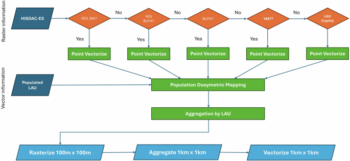
Workflow of population disaggregation model. Source: Own elaboration.
For each period, population grids were produced following a clear and concise volume-preserving dasymetric mapping approach at LAU level. So, for a given period we iterate over municipalities looking for population support in the sequential order shown in Fig. 1. Given a vector census layer of municipal boundaries and a HISDAC-ES raster layer, for a populated municipal polygon (source zone) we proceed as follows:
1.
If a particular municipality has information on the total building indoor area (RES_BIA), then we downscale population proportionally to RES_BIA.
2.
If there is no information on RES_BIA, but the municipality has residential building footprint area (RES_BUFA), then we downscale population proportionally to RES_BUFA.
3.
If there is no information on the previous variables, but the municipality has building footprint area (BUFA), then we downscale population proportionally to BUFA.
4.
If there is no information on HISDAC-ES for a given municipality, then we use the ESPAREL coordinates of population entities to redistribute the municipal population.
5.
As a last resort, if no other information is found, in neither HISDAC-ES or ESPAREL, we assign municipal population to the coordinates of the municipal capital.
This sequential process ensures that, for each municipality, we use the best information available at each point in time. Steps 4 and 5 are necessary because, for some municipalities, at the beginning of the 20th century we did not find support for the population in HISDAC-ES. It should be obvious that the process is carried out for each year and municipality sequentially.
Table 1 shows the percentage of municipalities and population by type of support on which to locate the population. Overall, the results are reasonably good. In 1900, 93% of the municipalities and 95% of the population find support in the most reliable variable, RES_BIA, and the percentage of municipalities or population for which we must use auxiliary information, as we do not find support for it in HISDAC-ES, is very low, reaching only 1% of the population in 1900, when we have to use the settlement coordinates from 1887. The results improve significantly over time, and from the middle of the 20th century onwards it is no longer necessary to use information external to HISDAC_ES. The results in Table 1 due to the variable RES_BUFA come entirely from the 51 municipalities of Araba/Álava, whose land registry does not provide information on the building indoor area in any of the census years.
In fact, if we had to identify areas with insufficient or inadequate representation, we would find them mostly in the Basque Country. Figure 2 shows the estimated inhabited cells, with a resolution of 1 km × 1 km, for the provinces of Bizkaia and Gipuzkoa in the census years 1900, 1940, 1981 and 2021, and we observe two different situations where the spatial information supporting the population distribution generates an inadequate and different contribution. These two cases represent the two most extreme situations we have found. On the one hand, the information for Bizkaia comes entirely from the footprint of the buildings (BUFA), without classification by use, which generates an excessive dispersion of the population visible in all the years, especially in 1900. On the other hand, the information for Gipuzkoa is much more deficient, and in 1900 it comes largely from settlements coordinates of the of 1887 census, which generates an excessive concentration of the population in a few cells at the beginning of the 20th century. This phenomenon is also observed in 1940 and gradually disappears as the 20th century progresses. It is important to remember that the cadastres of these two provinces are different, in the data model and in the informational content.
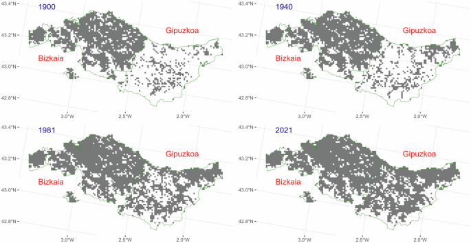
Inhabited cells, 1 km × 1 km, of the estimated population grid for 1900, 1940, 1981 and 2021 and the provinces of Bizkaia and Gipuzkoa (HIPGDAC-ES). Source: HISDAC-ES, Census 1900–2021 (INE), ESPAREL and own elaboration.
These situations are not generally observed in other regions. Figure 3 shows the same information as Fig. 2 for Madrid and allows us to observe a more realistic evolution in the populated cells. In this case, for almost all the municipalities we have information on the total building indoor area (RES_BIA) as early as 1900. Most regions show a pattern like that of Fig. 3, so the results seem similar in quality to HISDAC-ES, and although the overall results seem very plausible, there are areas where the final data produced may be more deficient. The population distribution algorithm stores intermediate information that allows tracking quality at the municipality level.
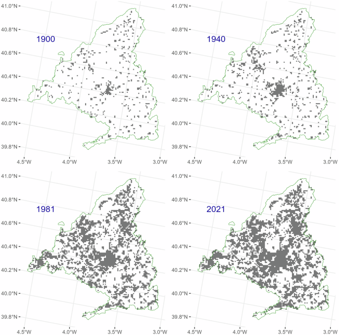
Inhabited cells, 1 km × 1 km, of the estimated population grid for 1900, 1940, 1981 and 2021 and the province of Madrid (HIPGDAC-ES). Source: HISDAC-ES, Census 1900–2021 (INE), ESPAREL and own elaboration.
The vector/raster dasymetric mapping approach is implemented at municipality level on the original resolution of the HISDAC-ES raster layers, 100 m × 100 m, using methods very close to the production of the GHSL population grids15, following the workflow indicated in Fig. 1. One important difference, overlooked in the literature, is that the population per cell is rounded to integer values at this resolution using LAU population as totals, –except for the 2011 census, whose population values published by INE are real–. The integer adjustment algorithm, performed at the 100 m × 100 m cell level, is the method of largest remainder18,19,20. Hence, population grids are integer valued at this resolution and aggregated afterwards to the standard resolution of 1 km × 1 km, in raster and vector formats.
Table 2 shows the population of each census and the number of inhabited cells estimated with the above algorithm. According to our estimates, while the population has multiplied by 2.5 in the period 1900–2021, the inhabited cells have only doubled.
A close inspection of Table 2 reveals some striking figures that deserve a few comments. The number of inhabited cells continuously increases up until the last two years, 2011 and 2021. In this case the last census, 2021, shows a significant drop in the number of inhabited cells compared to the previous census, 2011. One might think that this trend is due to the huge population growth between 2001 and 2011, as opposed to the low population growth between 2011 and 2021. However, this is not the case. It is easy to show that the result is, in a way, a statistical artifact derived from the fact that the INE published population data in real figures for the 2011 census, which as INE10 itself acknowledges was not a good idea and introduced additional complications. Our estimates maintain the INE population structure, and therefore the layers generated provide population figures in integers at the 100 m × 100 m cell level for all years except 2011, where the results of the disaggregation process are not rounded. The result is that the population in real figures overestimates the number of inhabited cells. If for 2011 we round off the population figures to integers at the 1 km × 1 km cell level, then the population obtained is 46,815,735 persons, slightly different from the total census population –Table 1–, and the number of inhabited cells would be 143,974, much more in line with the trend observed in Table 2. Even in this case the number of inhabited cells would be slightly lower in 2021 than in 2011 but given the magnitude of the differences we cannot rule out that this would not be the case if the rounding were done at the level of 100 m × 100 m cells.
Another curious fact, which is not possible to observe only with the information in Table 2, is that the trend observed for the years 2011 and 2021 in our estimates is radically different from that observed when we compare the only two population grids published by INE, derived by bottom-up procedures, and which correspond to the 2011 and 2021 censuses, where the inhabited cells in 2021 practically double those that existed in 201121. As indicated in Goerlich21, section 5, this is due to a design effect in the generation of the 2011 grid, which makes it unreliable for determining the actual number of inhabited cells in Spain in that year.