
The proposed optimized stacked-LSTM model’s primary objective is to accurately identify people’s opinions regarding cryptocurrency investment. The presented model has the capability of multiple stacked LSTM layers with optimized parameters that can effectively predict people’s sentiment for future crypto investments. Existing models are generally labeled as “less-generalized” since they tend to have difficulty applying what they learned to other scenarios that are not enclosed within their specific training data or domain. This further emphasizes the need for a better, more flexible and context-aware model that can effectively manage the variety and complexity of real-world data, especially in dynamic environments like social media. Some reasons that describe these models as less general are overfitting training data, narrow data reliance, insufficient contextual understanding, limited robustness, domain-specific limitation, and biases in training data, and challenges with transfer learning.
Figure 1 shows the deep architecture of the proposed model with a step-by-step procedure. This model has completed in various steps. Each step is filled with advanced Artificial Intelligence (AI) associated computations such as feature extraction, dimensionality reduction, multiple layering of the neural network, and nature-inspired PSO optimization. Initially, live Tweets are collected regarding the latest cryptocurrencies. Before applying the neural model to the \(Tweets \, [t_{1} ,t_{2} ,t_{3} ………………t_{n} ]\) corpus, noise reduction has been performed, like punctuation, whitespace, numbers, and URL removal. After removing noise from the dataset, it is tokenized in the form of \({\text{Corpus }}[w_{1} ,w_{2} ,w_{3} ………………w_{n} ]\). The essential feature engineering has been applied, namely N-Gram, Part-of-Speech (PoS) tagging, and sentiment word extraction to focus on the utility features. Dimensionality reduction is necessary for solving the AI model’s overfitting problem. Therefore, Principle Component Analysis collects the critical Principle Components (PCs) from the large sample. Finally, Glove word embedding is applied to generate the global word vectors \({\text{vect }}[v_{1} ,v_{2} ,v_{3} ………………v_{n} ]\). After that, the multiple layers of the LSTM neural network have trained on the worldwide vector \({\text{vect }}[v_{1} ,v_{2} ,v_{3} ………………v_{n} ]\) with PSO-optimized hyperparameters. Ultimately, the knowledge-enriched model has been produced to mine the opinion and predict Cryptocurrency’s future. The proposed model input sentences sequentially, one token at a time. Each word or phrase is represented as a vector (via embeddings), and the LSTM updates its internal state based on the current input and its previous state. This enables it to accumulate information about preceding words, phrases, and their relationships. This means that, by incrementally updating its internal state and learning what to retain or discard, an LSTM can capture meaningful relationships between phrases, even across long sentences. LSTMs are much better than traditional RNNs at maintaining relationships over longer distances, such as connecting “If–then.” structures in a sentence.
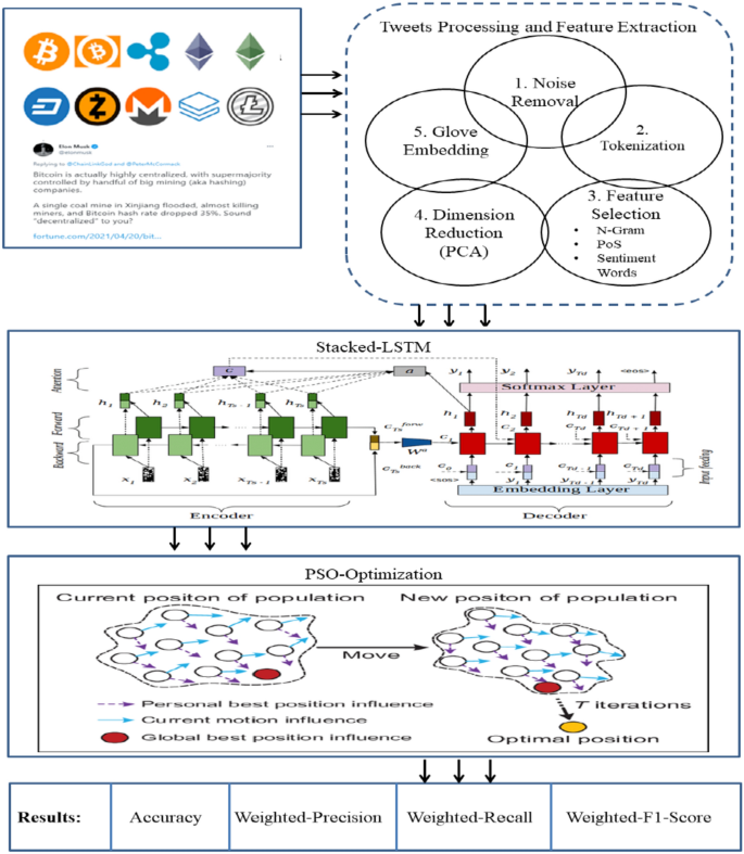
The Architecture of the proposed PSO-optimized staked-LSTM model for cryptocurrency price prediction.
Data engineeringData elicitation
The 9,998 cryptocurrency-associated unlabelled tweets have been collected from Kaggle.com to predict people’s sentiment towards Cryptocurrency. The Text-Blob corpus method is exploited to label the tweets as Positive, Negative, and Neutral. The polarity and subjectivity score are also calculated to get a deeper insight into the tweets. Table 1 presents the sample of the selected cryptocurrency tweets dataset.
The sentences in the text that relate to Twitter data seem clear, but can be improved for readers with different expertise levels. However, informal language that defines a tweet may be full of hash tags, mentions, and abbreviations, making it unclear for a reader with little technical background. Several pre-processing steps have been used in this work to enhance the clarity of the sentences including text cleaning, hash tag removal, emoji to text conversion handling abbreviations and slangs.
Data processing
Tweets are generally a composition of incomplete expressions containing noise, poorly organized sentences, irregular grammar, frequent acronyms, and non-dictionary phases. The unstructured content degraded the performance of sentiment classification. Therefore, refining the tweets before training the model is required, which is done in various stages.
Noise removal: This phase includes numbers, Non-ASCII characters, URL links, punctuation removal, and harmful reference replacement.
Part-of-Speech (PoS) Tagging: Provides elementary information to identify aspect terms. It includes categorizing the words in a text corpus with a particular part of speech based on their definition and context. Table 2 describes the tagging of speech presented in sentences.
Part-of-Speech
Tag
Noun
n
Verb
v
Adjective
a
Adverb
r
Review:
But
the
staff
was
very
horrible
to
us
Cluster-ID:
00101
01010
11,010
01100
00101
11,101
01110
01111
Semantic Orientation (SO): It measures how much the word is associated with positive and negative sentiment. PointWise Mutual Information (PMI), a measure of association of token t with respect to positive and negative reviews.
$$SO(t) = PMI(t,pos{\text{Re}} v) – PMI(t,neg{\text{Re}} v)$$
(1)
$$PMI(t,neg{\text{Re}} v) = \log \frac{{freq(t,neg{\text{Re}} v)*N)}}{freq(t)*M}$$
(2)
where \(freq(t,neg{\text{Re}} v)\) is the frequency of term t in a negative tweet, \(freq(t)\) is the frequency of t in the corpus, \(M\) is the number of tokens in a negative review, and \(N\) is the number of tokens in the corpus 27.
GloVe Embedding: For generating the co-occurrence matrix, GloVe incorporates global statistics to obtain word vectors. The central principle of GloVe is that the co-occurrence ratios between two words in a context are strongly connected to form a meaning.
Normalization: For scaling the vectors in uniformity, min–max normalization is performed on the dataset. [Eq. 3] presents the formulation of min–max normalization.
$$V^{\prime} = \frac{(V – \min )}{{(\max – \min )}}$$
(3)
\(V\) The set of attributes \(\max\) denotes the maximum value from the attributes, and \(\min\) represents the minimum value in the dataset’s attributes \(V^{\prime}\). Represents the normalized data that holds values from 0 to 1.
Figure 2 presents the text length of positive, negative, and neutral tweets. The above pre-processing steps enrich the tweets for building an efficient sentiment classification model. The text content is further converted into a co-occurrence matrix as an input for the Stacked-LSTM model28.
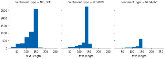
The Text Length Count of Neutral, Positive, and Negative Tweets.
Stacked LSTM
LSTM is the extended version of RNN introduced by Hochreiter and schmidhuber29. It overcomes the problem of RNN and can handle the long dependencies between phrases. The stacking of multiple layers of LSTM arranged hierarchically in a single model allows one layer to pass the output to the next in sequence, with each layer being able to detect more complex patterns and temporal dependencies at different levels of abstraction. The first LSTM layer receives the input sequence, such as a time series or a sentence, directly and analyzes this input to capture fundamental dependencies and patterns like trends or short-term fluctuations in time-series data or local context in text. The output from this layer includes hidden states and cell states for each timestep, which carry information on the dynamics of the sequence. Each subsequent LSTM layer takes hidden states from the previous layer rather than raw input data as an input. Therefore, these layers can process information already analyzed, meaning they can be able to learn higher-level abstract features. In this case, while the first layer may depend on local dependency, the second layer could point out longer dependency. The deeper layers usually focus on more complex or long-range patterns in the data, which improves the model’s ability to understand intricate relationships within the sequence.
The LSTM embedded three major gates, namely forget gate (\(f_{t}\)), input gate (\(i_{t}\)), and output gate (\(o_{t}\)). These manage the flow of information for updating, writing, and reading in the network. [Eqs. 4, 5, 6, 7, 8, 9] presents the mathematical evaluation of LSTM30.
$$f_{t} = \sigma (W_{f} [h_{t – 1} ;x_{t} ]) + b_{f}$$
(4)
$$i_{t} = \sigma (W_{i} [h_{t – 1} ;x_{t} ]) + b_{i}$$
(5)
$$o_{t} = \sigma (Wo[h_{t – 1} ;x_{t} ]) + b_{o}$$
(6)
$$\tilde{c}_{t} = \tanh (Wc[h_{t – 1} ;x_{t} ]) + b_{c}$$
(7)
$$c_{t} = i_{t} \otimes \tilde{c}_{t} + f_{t} \otimes c_{t – 1}$$
(8)
$$h_{t} = o_{t} \otimes \tanh (c_{t} )$$
(9)
$$H = [\vec{h}_{t} :\mathop{h}\limits^{\leftarrow} _{t} ]$$
(10)
where,\(h_{t}\), \(c_{t}\), and \(x_{t}\) are the hidden vector, cell state, an input vector. \(W_{f} ,W_{i} ,W_{o} ,W_{c} ,b_{f} ,b_{i} ,b_{o} ,b_{c}\) Are the weight matrix and bias vectors for each gate. For encoding, the sequence in backward and forward Bidirectional-LSTM is formulated in [Eq. 10]. The proposed model stacked multiple LSTM layers for effective result manipulations.
Due to the ability of this architecture to tackle complex sequential data is impressive, using this stacked-LSTM architecture in sentiment analysis has several benefits.
Deeper Understanding of Text: A stacked-LSTM, with multiple LSTM layers, enables the model to learn hierarchical features of text data. Lower layers capture simpler patterns, while upper layers capture higher-level abstractions.
Improved Contextuality: Hierarchical representation facilitates the model to pick up subtle sentiment shifts in long texts or complex sentences.
Improved Expressive Power: Every level in an LSTM is a degree of non-linearity, allowing stacked architecture to express complex word phrase relationships which underlie sentiment.
Flexibility and Scalability: Stacked-LSTMs may be adapted based on the nature of the complexity of the data by changing the number of layers and hidden units. For very large datasets or tasks with rich sentiment patterns, deeper architectures could be more helpful.
Latent contextual semantic features refer to the underlying or implicit meanings of words that can be understood from their context within a sentence, paragraph, or larger document. These features are crucial because the meaning of a word often relies on the words around it and the broader context in which it appears. Words can take on different meanings based on their context. For instance, “cool” can signify “cold” or “impressive” depending on how it’s used in a sentence. Contextual semantic features assist the model in grasping these nuances. The sentiment of a sentence can be shaped by the context in which a word is used. For example, “I love the concept but hate the implementation” includes words like “love” and “hate,” yet the overall sentiment is complex and requires context to fully understand the mixed feelings. By employing techniques such as word embeddings (like Word2Vec, GloVe, or contextualized embeddings like BERT), the model can uncover the deeper semantic connections between words. For example, it can learn that “happy” and “joyful” are semantically similar and convey a positive sentiment.
Attention mechanism
The attention mechanism is applied to gather the more profound context information present in the tweets. It focused on the local level and global levels. The local level pays attention to only a few words of sequence, and the global level pays selective attention to all the words available in the sequence. This paper applied local attention and focused on the small width of sequence \(S = \{ x_{1} ,x_{2} ,……..x_{n} \}\) and \(h_{i} = [h1,h2,…………,h_{n} ]\) hidden word vectors calculated from sentences.
$$_{{h_{{t,t^{t} }} = \tanh (x_{t}^{T} * W_{t} + x_{{t_{t} }}^{T} * W_{t} + b_{t} )}}$$
(11)
$$_{{e_{{t,t^{t} }} = \sigma (x_{t}^{T} * W_{a} + x_{t} * W_{t} + b_{a} )}}$$
(12)
$$a_{t} = soft\max (e_{t} )$$
(13)
$$l_{t} = \sum\limits_{{t^{t} }} {a_{{t,t^{t} * x_{{t^{t} }} }} }$$
(14)
The multiplicative attention of the given sequence is generated in [Eqs. 11, 12, 13] and normalized by [Eq. 12]. After that, the context vectors of the normalized sequence are calculated in [Eq. 14]. The main differences between latent contextual semantics and co-occurrence statistical features lie in how they model relationships between words, the kind of information that they capture, and their applications in NLP.
Latent Contextual Semantics: The hidden meaning or relationship that is implied by the context in which words or phrases are used. In it, the goal is to understand the semantic relationship between words through the use of their context. Captured using advanced models such as embeddings (word2vec, glove, BERT), or other contextual representations.
Co-occurrence statistical features: These are statistical relationships between words based on the frequency of their simultaneous appearance in a given corpus. They focus on the surface patterns of word usage without attempting to model deeper semantics; thus, they are often captured using techniques such as co-occurrence matrices, Point-wise Mutual Information (PMI), or word frequency counts.
PSO optimization
The next step is featuring selection, which is done by applying the greedy PSO algorithm. PSO is one of the effective techniques for calculating the optimized features from noisy subsets. It is biologically motivated and inspired by a horde of birds searching for food. Each individual in the dataset represents a bird that holds the fitness value in the search space. In this case, it has a best-labeled lexicon, and the possible solutions are called the particles that are the parts of the population. Every particle keeps its best solution called as \(pbest\). At the same time, the best value selected from the whole swarm is called as \(gbest\). Figure 3 presents the velocity and position relationship in PSO.
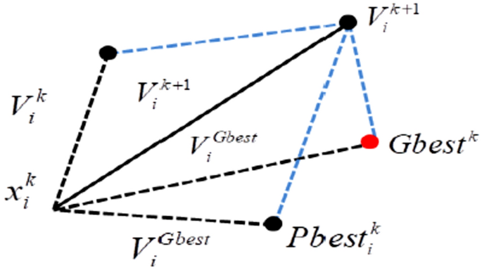
Relationship of PSO within velocity and position vectors.
Majorly, PSO works on the principle of updating position and changing velocity. In the first step, every particle changes its velocity towards its \(pbest\) and \(gbest\). In the second step, the particle updates its position. Every particle in space is represented as \(D – \dim ension\) a vector. The nth vector can be represented as \(A_{n} = (a_{n1} ,a_{n2} ,……….a_{nD} )\). The velocity of the nth particle can be represented as \(V_{n} = (v_{n1} ,v_{n2} ,……….v_{nD} )\) where the best previous position of a particle can be represented as \(P_{n} = (p_{n1} ,p_{n2} ,……….p_{nD} )\).
Particle Swarm Optimization is a population-based optimization algorithm based on the social behavior of birds and fish. It is applicable for searching through the space of hyperparameters in LSTM layers in a systematic manner to get the best values together. Table 2 represents the steps of PSO for LSTM hyperparameter tunning.
The PSO has a number of advantages over traditional optimization techniques, especially in complex and high-dimensional problems. Some of the key advantages are as follows:
Ease of Implementation and Simplicity: PSO is relatively simpler to implement and understand compared to other optimization algorithms, such as GA or SA.
Robustness to Non-Linear, Multimodal, and Complex Objective Functions: PSO can solve complex, nonlinear, and multimodal optimization problems effectively, such as those difficult to solve by the traditional gradient-based algorithms.
Parallelism and Global Search Ability: In PSO, every particle is an independent agent that computes its position and updates its state according to the experiences it gains and its neighbors. In this manner, a large number of particles can be concurrently exploring the search space in the pursuit of a global optimum.
Low Requirement of Derivatives: Unlike gradient-based optimization methods, PSO does not require the derivatives of the objective function to be known or continuous.
Sentiment classification using aspect category
The Softmax classification layer is applied in the proposed model to classify cryptocurrency tweets. This layer receives the input from the local attention layer and calculates the probability score of each sentiment label and aspect category. After that, the aspect category and sentiment label are predicted as follows in [Eq. 15].
$$\hat{y} = soft\max (W * l_{t} + b)$$
(15)
$$w_{t + 1} = w_{t} – \alpha m_{t}$$
(16)
$$m_{t} = \beta m_{t – 1} + (1 – \beta )\left[ {\frac{\delta L}{{\delta w_{t} }}} \right]$$
(17)
Here \(b\) \(W\) and are the bias vectors and weight matrix. The categorical cross-entropy loss function is exploited with Adam weight optimizer to measure the loss of the model in Eqs. 16, 17. Where, \(m_{t}\) is the gradient at time \(t\), \(m_{t – 1}\) is at time \(t – 1\).\(w_{t}\) is the weights at time \(t\), \(\alpha_{t}\) is the learning rate, and \(\beta\) represents the moving average parameter [constant 0.9].
Challenges in model training
The Particle Swarm Optimization (PSO) process for a stacked LSTM architecture has its own problem in hyperparameter optimization.
High-Dimensional Search Space: Hyperparameter optimization for stacked LSTMs has a high-dimensional search space. It includes parameters such as the number of layers, number of units per layer, learning rate, dropout rate, and batch size. PSO finds it difficult to explore and exploit such a large space efficiently.
Particle Initialization: Ineffective initialization of particles may cause them to not explore the search space effectively.
Loss Function Sensitivity: The optimization process is highly dependent on the loss function. PSO may have difficulty with noisy or non-smooth loss landscapes.
Stochastic Behaviour: The PSO is a stochastic algorithm. Results between runs may not be the same due to randomness in initialization and updating. Run multiple times and take the average value to ensure convergence.