Magnetic susceptibility varies between 20 × 10−5 and 30 × 10−5 S.I. with peaks of up to 239 × 10−5 (Fig. 2). Saturation remanent magnetisation (Mrs) varies between 0.89 mAm2/kg and 13.7 mAm2/kg with an interval of variable values between 15 ka and c. 13 ka as shown by magnetic susceptibility. Coercivity of remanence (Bcr) is low overall (c. 35 mT) except for the 15–13 ka high variability interval (40–60 mT, Fig. 2). First Order Reversal Curve (FORC) analyses revealed three dominant magnetic signatures. Type A (Fig. 3, samples 3,4,5 and 7) have a narrow central ridge between 10 and 80 mT with limited vertical spread indicating Single Domain (SD) particles with little magnetostatic interactions7. Our choice of field spacing during analyses (2 mT) limits how narrow the ridge will appear on FORC diagrams. Type B (Fig. 3, samples 1–2) have a broader ridge between 0 and c. 40 mT peaking at Bc ≈ 20 mT. Type C samples (Fig. 3, samples 6 and 8 and Fig. 4) have FORC diagrams with an oval central peak centred at Bc ≈ 60–70 mT and Bu ≈ −5 mT, with significant vertical spreading typical of strongly interacting SD particles. Hysteresis analyses of schist, grey glacial clay, silt deposits and regolith/soil from around the lake revealed very low concentrations of magnetic minerals with low coercivity, superparamagnetic grains or multidomain grains (Fig. 5). FORC analysis was conducted on the sample which appeared to have the highest concentration of magnetic minerals, but the data were too noisy to allow characterisation of magnetic minerals (Sample 3, Fig. 5C) except for a faint multidomain signature in Sample 6 (Fig. 5D). X-ray Fluorescence (XRF) ratios Fe/Ti and Mn/Fe (Fig. 2), are divided into an upper section (above c. 300 cm) with limited variability and lower section (below 300 cm) with high amplitude variations and prominent peaks in Mn/Fe.
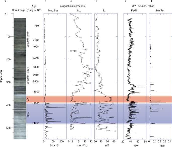
a Condensed core image with radiocarbon ages. Laminated grey silt dominates below 380 cm with a gradational shift to diatomaceous olive-green mud above 380 cm. b “Mag Sus” is the magnetic susceptibility, and (c), Saturation remanent magnetisation (Mrs) and (d), Coercivity of remanence (Bcr) are the saturation remanent magnetisation and the coercivity of remanence derived from Isothermal Remanence Magnetisation (IRM) data, respectively. X-ray Fluorescence (XRF) elemental ratio (e), Fe/Ti indicates whether sediments have been affected by Fe reduction and (f), Mn/Fe indicates the degree of water column oxygenation where high values indicate poor oxygenation.
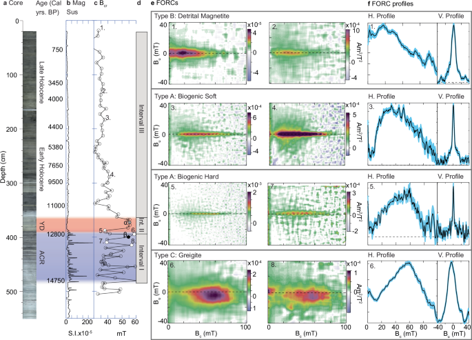
a Condensed core image with radiocarbon ages (b), “Mag Sus” is the magnetic susceptibility and (c), Coercivity of remanence (Bcr). d Core divisions discussed in the text, and (e), First Order Reversal Curve (FORC) diagrams with corresponding (f) vertical and horizontal profiles of the three FORC morphologies (categories): Type A — biogenic soft and hard magnetite, Type B — detrital magnetite, and Type C — greigite. High resolution FORCs for samples α and β are in Fig. 4.
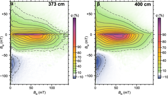
α and β show details of the magnetic signature of two greigite-bearing samples: α from the Younger Dryas and β from the ACR. The First Order Reversal Curve (FORC) diagram is dominated by oval central peak at 60 mT indicating the presence of greigite with the addition of a thin central ridge indicative of biogenic particles (magnetofossils).
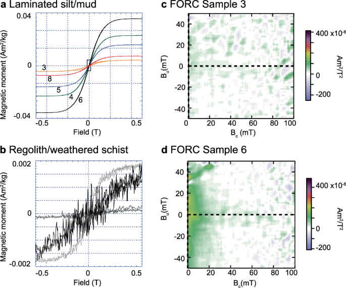
a Hysteresis data of laminated silt and mud deposits which crop out above the modern level of Lake Hayes. b Hysteresis data of schist and weathered schist showing very low concentrations of magnetic minerals. c, d are FORC analyses of samples 3 and 6 from (a) with low magnetic mineral concentration resulting in poor quality FORC data.
FORCs allow the identification of mixtures of magnetic particles because they simultaneously provide information on domain state, coercivity, concentration, and magnetostatic interactions8. We identified three distinct magnetic mixtures (Fig. 3):
Type A: Biogenic magnetite
Type A FORCs are characterised by a narrow central ridge, which is typical of noninteracting, single-domain biogenic magnetite. These particles are produced by magnetotactic bacteria, a broad group of motile prokaryotes that synthesise iron-based minerals known as magnetosomes9 which they use to navigate (known as magnetotaxis)10. These bacteria have been observed to ‘swim’ in the direction of the local geomagnetic field11, and their magnetosomes (magnetofossils) have been identified in sediments ranging from abyssal marine12 to fresh water13. In microoxic environments, they produce magnetite (Fe3O4), which is the most commonly identified biogenic magnetic mineral12,13. Biogenic magnetite has been further subdivided into biogenic hard and soft from coercivity spectra14, where coercivity differences have been linked to magnetosome morphology15,16. In Lake Hayes samples, horizontal profiles through the central ridge (Bu = 0) indicate that both biogenic hard and soft components are present with a peak response between 20 mT and 60 mT, followed by a gradual decay to 80 mT. Biogenic Soft magnetite appears to be confined to the upper part of the core (Fig. 3 samples 3 and 4), and Biogenic Hard magnetite (Fig. 3 samples 5 and 7) is in the lower part of the core.
Type B: Detrital Magnetite
Is identified by the overlap of a low-coercivity central ridge peaking at or near Bc = 0 on the horizontal profile and a broad base with increasing vertical spread towards Bc = 0 on the vertical profile. The overall coercivity is lower than Type A samples (the peak in the horizontal profile occurs at 20–30 mT, Fig. 3, samples 1 and 2). Type B FORCs indicate magnetite grains with a broad grain size distribution ranging from superparamagnetic to pseudo-single domain17, which we suggest are either sourced directly from surrounding schist or from erosion of soils.
Type C: Greigite
Care must be taken when interpreting FORCs from samples with mixed populations of SP and SD grains because peak coercivities can range widely from c. 70 mT for SD grains to zero for SP grains18. Type C FORC diagrams display an oval central peak at c. 60 mT, which indicates the presence of natural single domain (SD) greigite with substantial magnetostatic interactions19 (Fig. 3, samples 6, 8, and Fig. 4 α and β). Greigite (Fe3S4) is a thiospinel which, in sedimentary environments, can form rapidly during reduction diagenesis20,21. If sufficient reagents are present, the diagenetic reaction will lead to paramagnetic pyrite (FeS2). However, when reagents are limited, intermediate phases such as ferrimagnetic greigite, can form22. An alternative interpretation is that Type C FORCs contain monoclinic pyrrhotite (Fe7S8), however, the coercivity range of this mineral extends beyond the range of the horizontal profiles, and pyrrhotite FORCs have a less oval profile19. Furthermore, pyrrhotite is unlikely to form in low-temperature aqueous reducing conditions23 and is more likely to be of detrital origin (i.e., eroded from basement rocks). The basement rocks of the Lake Hayes drainage basin are Caples and Rakaia terrane schists, which have been reported to contain metamorphic magnetite and minor pyrite and pyrrhotite24. In the Wakatipu basin, coarse (> 3 mm) detrital magnetite is abundant in the Arrow River sediments immediately north of Lake Hayes and in metavolcanic horizons in greenschist facies rocks24. Magnetic analyses of basement schist, glacial deposits, soils and regolith from the lake catchment identified only magnetite (Fig. 5). Therefore, we suggest that magnetic mineralogy of Type C samples is dominated by greigite formed in situ under reducing conditions.
High-resolution FORC analyses of two samples, one from within the Younger Dryas (Fig. 4, sample α at 373 cm) and one from the ACR (Fig. 4, sample β at 400 cm), were carried out to understand better the magnetic mineral compositions. Both analyses revealed an oval central peak centred at c. 60 mT, which is typical of sedimentary greigite, but they also contain the thin, narrow central ridge which is typical of biogenic magnetic particles (magnetofossils). The biogenic contribution, identified with the central ridge, remains relatively stable (from 0.109 mAm2/kg in α to 0.129 mAm2/kg in β, see supplementary table) with identical coercivity distribution in both samples, while the authigenic (abiotic) greigite concentration, identified with the remaining FORC contributions, increases (from 2.03 mAm2/kg in α at 373 cm to 5.40 mAm2/kg in β at 400 cm).
In sulphide-reducing environments9, biogenic greigite can also be produced by bacteria which have so far been divided into many-celled prokaryotes9,25 and large rod-shaped bacteria26. The magnetic properties of biogenic greigite are poorly understood but appear to be similar to those of biogenic magnetite27. However, because the co-existence of biogenic magnetite and greigite is in essence, impossible24, it is reasonable to interpret the narrow central FORC ridge observed in Type C samples as being the signature of biogenic greigite.
Interpretation of magnetic mineralogy
Based on FORC results and magnetic characteristics, we divided the core into three intervals: a lower interval between 480 to 390 cm (Fig. 3, Interval I), a central interval between 390 cm and 360 cm (Fig. 3, Interval II) and an upper interval between 360 cm and the core top (Fig. 3, Interval III).
Interval I – The Antarctic Cold Reversal (480 cm to 390 cm)
The radiocarbon age model indicates that sediments between 480 cm and 390 cm (Interval I) were deposited during the ACR. Because the working half of the core was destructively sampled after magnetic susceptibility measurements were made and several years elapsed until magnetic mineralogy samples were collected from the archive half, the alignment and correlation of magnetic susceptibility with Mrs/Bcr data was made difficult.
Magnetite and greigite have very similar magnetic susceptibility values of 5.8 × 10⁻⁴ m3 kg−1 28 and 3.2 × 10⁻⁴ m3 kg−1 29 respectively therefore we suggest magnetic susceptibility is not mineralogy sensitive in this interval.
However, because Mrs data are primarily concentration-dependent (like magnetic susceptibility), we suggest that during the ACR, high Mrs and magnetic susceptibility is associated with greigite, while low Mrs and magnetic susceptibility are associated with magnetite intervals.
The fluctuations in magnetic susceptibility, coercivity and magnetic mineral concentrations recorded during the ACR can be interpreted as follow: High coercivity (Bcr) samples have high Mrs, and Type C FORCs indicative of greigite. The alternate low coercivity samples have low Mrs, and Type A FORCs indicative of biogenic magnetite.
Magnetotactic bacteria reside in the water column at the oxic-anoxic transition zone9 or, in the case of well-oxygenated bottom waters, beneath the sediment-water interface. We suggest the presence of biogenic magnetite recovered in the sediments indicates that the lake was aerobic. Greigite samples on the other hand indicate reducing or anoxic conditions either during sediment deposition (i.e., greigite was produced at the sediment-water interface), or after deposition.
The FORC signature of the Type C samples suggested the presence of both biogenic and authigenic greigite. We, therefore, suggest that greigite formation begins with magnetotactic bacteria before the onset of the abiogenic greigite formation, owing to their biomineralizing capabilities at very low iron concentrations. We suggest that greigite in Lake Hayes was produced syndepositionally or near-syndepositionally under the anoxic conditions of the lakebed, regardless of whether greigite was precipitated biologically or chemically. If greigite had formed long after deposition deep in the sediment column, we would not expect it to be confined to thin intervals (
We interpret the oscillations between greigite (Type C samples) and biogenic magnetite (Type A samples) below 390 cm as reflecting alternations between oxic and anoxic conditions. The Fe/Ti ratio in XRF data supports this interpretation because it indicates selective depletion of iron-bearing minerals relative to titanium-bearing minerals (Fe is prone to dissolution during reduction while Ti is not). Prior work in lacustrine systems30 showed that the Mn/Fe ratio is also a useful redox indicator because Mn is relatively more mobile under anoxic conditions and is more sensitive to redox changes than Fe. Accordingly, the varying Mn/Fe ratio in the Lake Hayes record provides additional evidence for episodic changes in the redox state of lake water. However, partitioning of Fe and Mn in aquatic systems is complex and can be influenced by a number of factors31 therefore a combination of complementary paleo-redox indicators should be used. In the case of the Lake Hayes succession, strong evidence of reducing conditions is inferred from the magnetic mineral assemblages combined with the selective depletion of iron-bearing minerals in the Fe/Ti XRF ratio, while peaks in Mn/Fe data may indicate oxygenation events. Previous research on magnetic variations in lacustrine sediments13 led to the suggestion that lakes can experience oscillations between oxic and anoxic states, where oxygen levels become depleted through excess nutrient load and productivity until a mixing event oxygenates the lake.
In temperate climates (between the polar or equatorial regions), lakes can experience annual temperature cycles that can result in thermal stratification. In winter months, for example, lakes can stratify if they become ice-covered and therefore isolated from the atmosphere or in summer months, reduced wind stress and solar surface warming, may also result in stratification32. In this setting, summer thermal stratification ends in the autumn period as the lake loses heat and wind stress increases. Other possible causes for lake stratification may be seasonal ice cover and variations in river input.
Unfortunately, due to very low sedimentation rates in the lake, the seasonal ice cover hypothesis can´t be tested as no observable fine-scale laminae that are typically deposited during prolonged winter ice cover33 could form. However, we consider that because of New Zealand’s maritime influence where warm air masses can penetrate the interior of the land mass at any time of the year, it is unlikely that significant winter ice cover occurred.
Multidecadal changes in river input as a driver for change in stratification or redox state in Lake Hayes are not supported by geochemical records during the ACR 3. However, because annual rainfall is intrinsically linked to the strength of the westerly winds in this sector of the Pacific 3 variations in river input would have a similar effect and be driven by the same process (i.e., more wind results in greater rainfall, higher inflow and more overturning).
We hypothesise that during the ACR interval, alternations in redox conditions recorded in the Lake Hayes sediment core were likely climatically controlled in a similar way as today, where seasonal bottom anoxia happens because of strong summer stratification (and excess nutrient supply) and is followed by winter mixing. We consider that biogenic magnetite intervals indicate enhanced mixing/overturning (more mixing from higher wind stress) periods, and greigite intervals indicate anoxia and stratification (less wind) periods. We suggest that winter wind stress and summer thermal stratification were the main controllers of the redox state of the deep lake waters.
Interval II – The Younger Dryas (390 cm to 360 cm)
The c. 30 cm interval between 360 cm and c. 390 cm (Interval II), corresponds to the Younger Dryas and is dominated by low Mrs, high coercivity, and Type C FORCs indicating the presence of greigite with the Fe/Ti data indicating pervasive Fe dissolution. We suggest this interval indicates persistent reducing conditions and that the lake was stratified and anoxic during the Younger Dryas. Supporting evidence comes from Ca/Ti data 3, which indicates increased carbonate production, which is typically linked to episodes of enhanced evaporation and possible lake closure (i.e., reduced inflow and no outflow)34.
Interval III – The Holocene (360 cm to core top)
Finally, in the upper c. 360 cm (Interval III), magnetic susceptibility has limited variability, while Mrs (Fig. 2) indicates a gradual upcore increase in magnetic grain concentration from c. 360 to c. 250 cm, after which Mrs decreases gradually up the core. Coercivity does not vary greatly, with an average Bcr of 36 mT. A gradual decrease in Bcr after 360 cm may indicate that the transition out of the Younger Dryas was gradual (occurring over several centuries) rather than abrupt. FORC analyses appear to shows an upcore shift from biogenic magnetite to detrital Type B magnetite-dominated mineralogy with supporting evidence for this gradual transition provided by the gradual decrease in Bcr values up core. We do not propose a mechanism for this gradual transition, except that it appears that environmental conditions became unfavourable for magnetotactic bacteria and the production of magnetosomes.
We conducted a spectral analysis of magnetic susceptibility and Fe-Ti XRF data from Interval I. Different age models were tested to include the errors associated with the top and bottom depths of Interval I. With a measurement interval of 5 mm in magnetic susceptibility data the shortest cycle (highest frequency) which can be resolved is 20 mm. When using the average age model, two cycles which exceed the 99% confidence limits are identified in the magnetic susceptibility, which have frequencies of 70 and 52 years (Fig. 6). If using the youngest age model, the cycles are 79 and 55 years and when the oldest age model is used the cycles have a period of 67 and 53 years. Regardless of which age model is used, the spectral peaks are well above the background noise level with a corresponding average Nyquist frequency of 12.8 years as reported by REDFIT. The average sedimentation rate for the entire core is c. 0.3 mm/yr and c. 0.45 mm/yr in Interval I. We did not identify statistically significant cycles in the Fe-Ti XRF data, which we attribute to significantly higher white instrument noise35.

Results of magnetic susceptibility data from Interval I using REDFIT-X. Data were converted to the time domain using radiocarbon dates, and Monte Carlo simulations were carried out to determine the confidence Intervals. Two cycles which exceed the 99% confidence limits are identified, which have frequencies of 70 and 52 years.