As part of last month’s Rankine Lecture, UC Berkeley’s Kenichi Soga presented case studies on how distributed sensing data and data analysis can lead to more adaptive infrastructure.
Kenichi Soga, who is currently Donald H McLaughlin chair in mineral engineering and a distinguished professor of civil and environmental engineering at University of California, Berkeley (UC Berkeley), gave the 63rd Rankine Lecture on the topic of “From geo-monitor to geo-adapt: leveraging distributed sensing and data analytics for performance-based design, construction and maintenance”.
The event was held at Imperial College London on 19 March.
He began the lecture by introducing a challenge for current infrastructure systems.
“We often design our infrastructure with a lifespan of 100 years, but some of our infrastructure has already exceeded this, and many of our infrastructure owners are increasingly looking to extend the life of their assets,” he explained.
“At the same time when we look at the demand side, the world around us is constantly evolving.”
In a city like London, for example, the social needs, environment and patterns of activity today differ significantly from those of 30 years ago – and they will likely continue to change over the next 30 years.
This means that ageing infrastructure is not only linked to material degradation but also changes in usage patterns, environmental conditions and climate.
“Given these uncertainties, infrastructure can be designed to be adaptive rather than assumed to be simply static,” Soga continued.
“The key is to understand the actual performance of our infrastructure.”
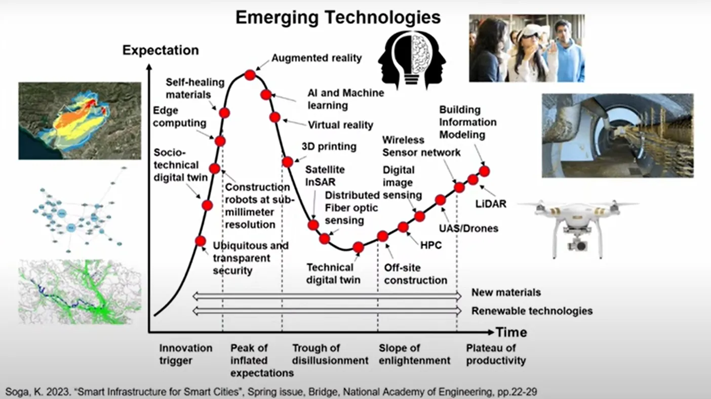
Emerging technologies – such as advanced sensors and data analytics – now make it possible to monitor infrastructure more effectively and gain deeper insights into system behaviour.
“In summary, we may have to embrace that our 100 years design life concept may not be compatible with actual demand in the future. This means we can think about making our infrastructure adaptive to change,” he said.
“Let’s imagine a world where future generations no longer have to worry about ageing infrastructure.”
Continuous monitoring
Soga’s focus for his lecture was geotechnical monitoring for detecting movements, particularly through distributed fibre optic sensing (DFOS).
According to Soga, DOFS is an emerging technology that is now progressing towards practical adoption within the infrastructure sector. However, its widespread uptake in the geotechnical industry will ultimately depend on the value it delivers to projects.
It enables continuous monitoring of strain, temperature, vibration and noise along the length of the fibre optic cable that can span many kilometres.
“Traditionally infrastructure design and maintenance rely on safety margins to account for uncertainties,” Soga noted.
He said that infrastructure performance naturally fluctuates, and in the conventional approach performance thresholds are established based on statistical distribution or engineering experience.
“However, in some cases an accident may happen and performance unexpectedly falls below the defined limit. When this happens, we recalibrate the threshold. Sometimes accidents may still occur due to previous unidentified mechanisms requiring further adjustments to these limits,” Soga said.
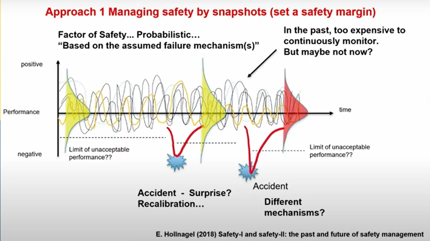
“In the past, continuous infrastructure monitoring was very expensive; however, with the advances in sensing technology continuous monitoring is now becoming economically feasible.”
Advancements in sensor technology and data analytics can now enable continuous monitoring and assessment of infrastructure performance.
Understanding actual performance enables:
Quick response if an event begins to unfoldManagement of future unknown demand by reducing unknown risksIdentification of potential improvements in the design and construction processesAnd from a circular economy perspective, resource conservation, component reuse and sustainable design.Observational method
Soga presented three different case studies during his lecture, on tunnelling, pipeline works and piling.
These examined how the soil profile and construction processes influence the performance of geotechnical structures. He also discussed how these assessed actual performance versus assumed performance to derive the underlying mechanisms that govern their behaviour.
“By acknowledging the uncertainty and improving our ability to anticipate performance, we can enhance decision-making in geotechnical engineering,” he said.
One of the key discussion points was the use of the concepts of “cautious” and “most probable”.
Thee were originally introduced within the framework of the observational method, introduced by the late professor Ralph Peck in the 9th Rankine Lecturer.
Soga listed the eight key components of the observational method – particularly focusing on the “most probable” and “most unfavourable” states – as:
Perform sufficient site investigationAssess most probable and most unfavourable conditionsEstablish design based on most probable on anticipated behaviour (Design A)Select monitoring parameters and calculate anticipated valuesCalculate values of most unfavourable conditionsSelect design modifications options (Design B) with Design AMonitor and evaluate actual conditionsModify design to suit actual conditions (adopt Design B if necessary).
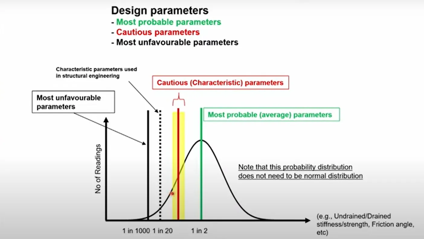
“Our engineering parameters, such as strength and stiffness, often exhibit statistical variability,” Soga explained
“Most probable is probably located in the 50th percentile. In contrast, the cautious value, which is commonly used in geotechnical design, is often set at approximate one standard deviation below the average. Most unfavourable scenario, which engineers may consider 1 in 1,000 probability or putting a factor of safety to the cautious parameters.
“In comparison, structural engineers who often deal with brittle materials may adopt a 1 in 20 value as a conservative estimate.”
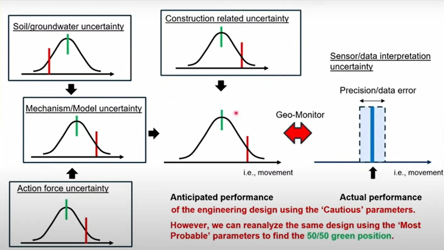
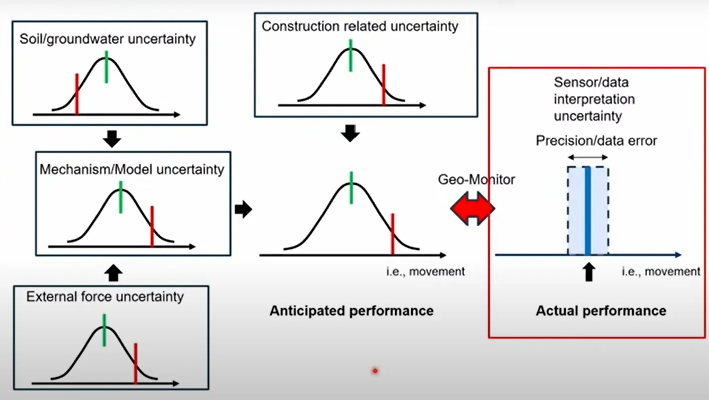
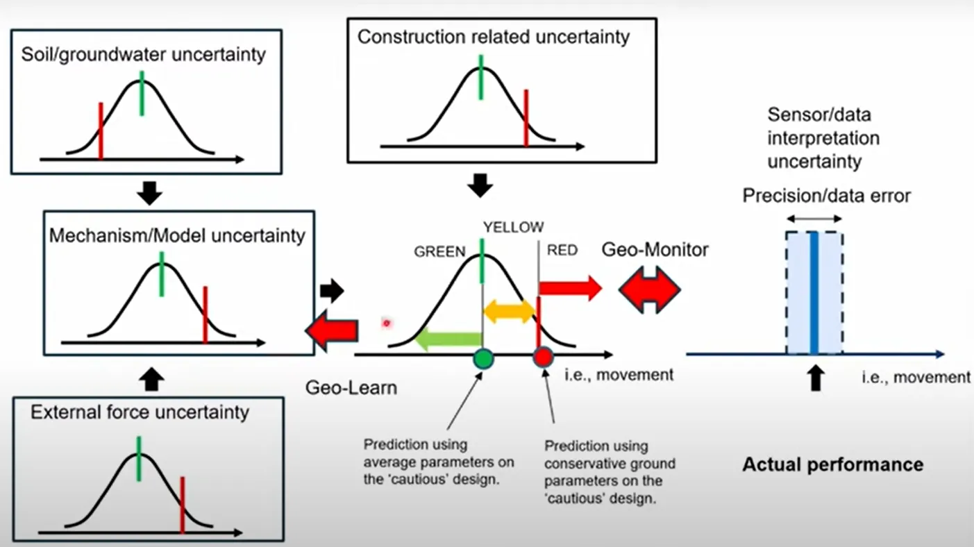
He continued: “In geotechnical engineering uncertainty extends beyond engineering properties. We must also account for uncertainty in action loads. There’s always uncertainty in selection and application of the mechanism or model and construction related activities.
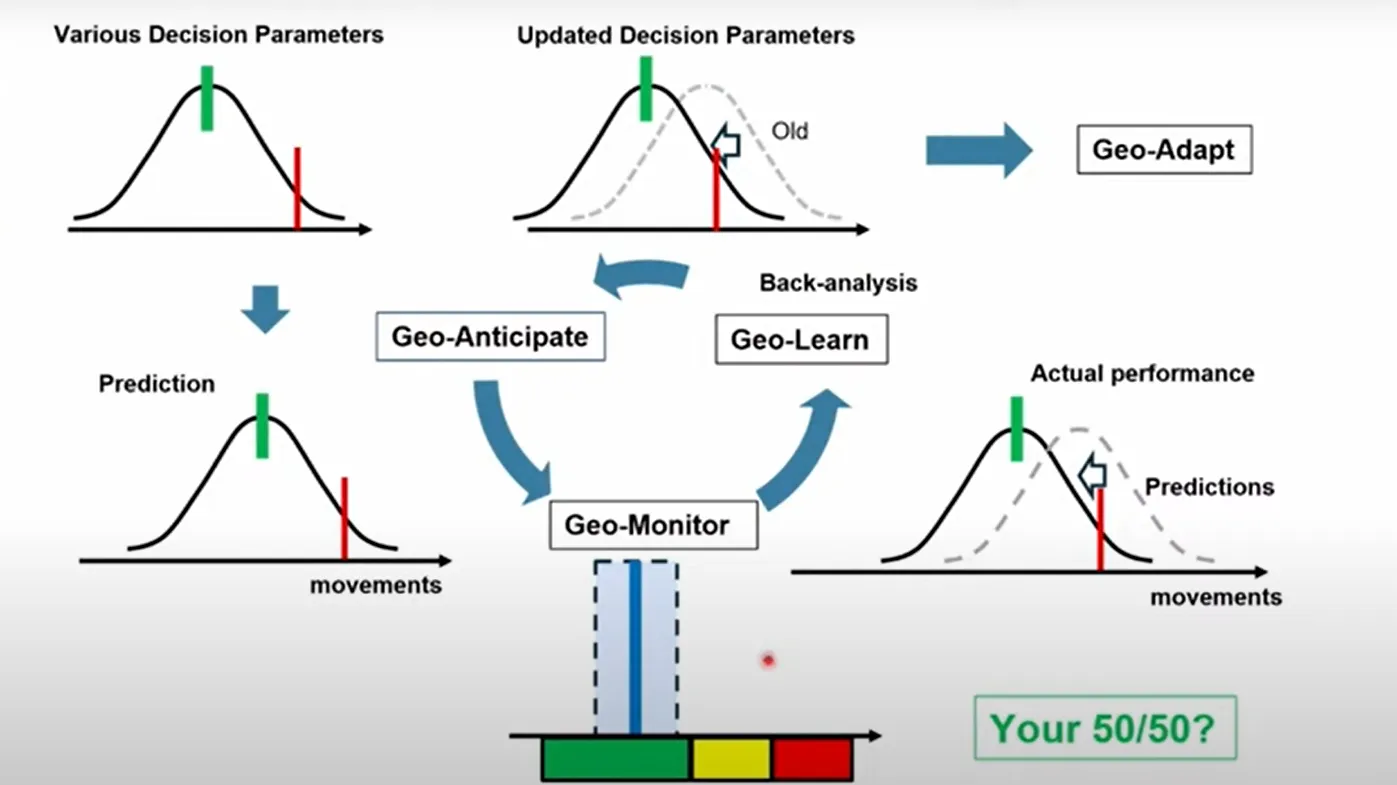
“Collectively, these factors influence the anticipated performance in terms of movement in this particular case. To address these uncertainties in design, we adopt cautious values, which are highlighted in red [see below graph] for all these uncertainties to predict the performance.
“We then conduct monitoring and compare the collected data against these predictions to ensure safety. The cautiously designed object with cautious engineering parameters will give the red prediction. However, we can re-analyse the same design using most probable parameters to find our 50/50 green position.”
In his talk, Soga aimed to demonstrate how emerging distributed sensing and data analytics technologies can contribute to this framework by seeking to understand the actual performance.
Buried infrastructure case study
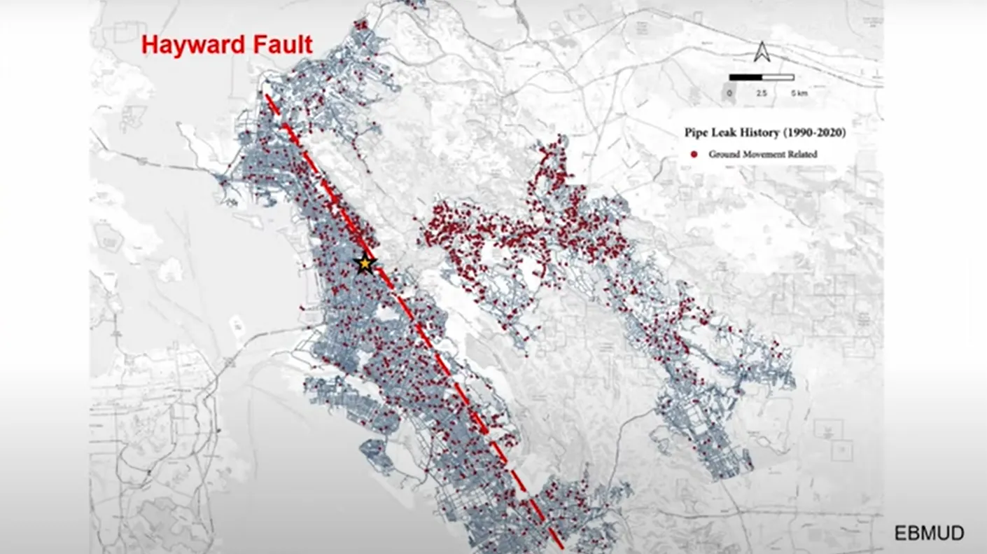
One of the case studies Soga presented was linked to pipeline performance in California’s East Bay area, where ageing infrastructure and ground movement pose significant challenges.
The East Bay water supply is managed by East Bay Municipal Utility District (EBMUD), the second-largest water utility in California. Some of the region’s oldest pipelines date back to the late 19th century.
EBMUD maintains approximately 6,700km of pipelines, which experience more than 1,000 annual failures, largely driven by ground movement and corrosion. The utility currently replaces only around 40km each year, meaning a full replacement cycle would take up to two centuries – far exceeding typical design life expectations.
“This raises a critical question or challenge: How can we develop more effective strategies for renewing our ageing infrastructure?” Soga asked.
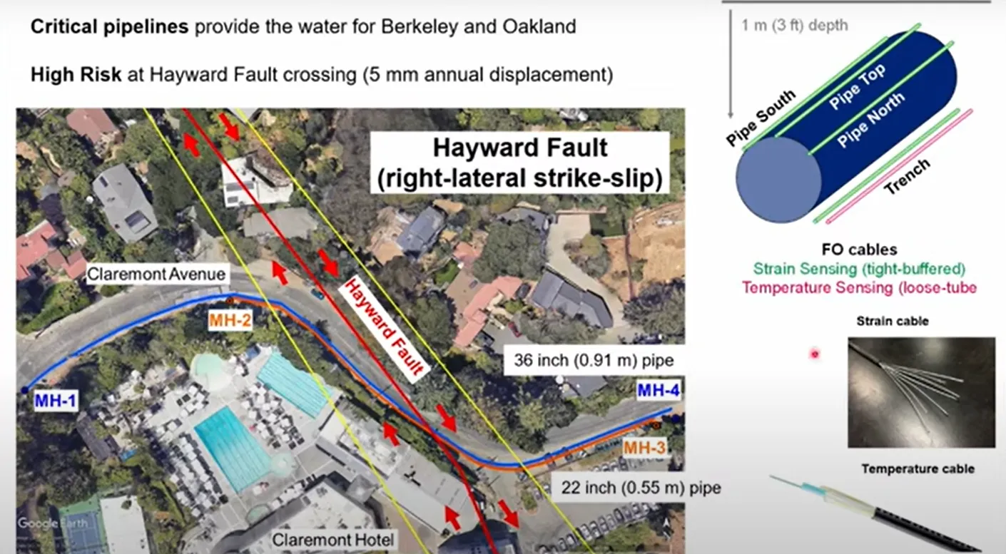
The case study centred on a pipeline supplying water to the UC Berkeley campus. This infrastructure crosses the Hayward Fault, a significant seismic feature running directly through the area.
In collaboration with EBMUD, researchers installed DFOS on two new high-density polyethylene (HDPE) plastic pipelines.
Three fibre optic cables were fixed along each pipeline: one at the crown and two at 45° angles from the horizontal. In addition, strain and temperature sensing cables were embedded within the trench.
During an 18 month monitoring period, the readings showed “tensile strain observed developing around the fault location, with the magnitude ranging from about 100 to 200 microstrain”, Soga said.
“The data revealed a pattern of tensile strain concentrated in the middle section of the pipeline where the fault is, and then we can start to create a mechanism of tensile deformation happening in the middle and small bending on the two sides.
“When recording is done, it is essential to assess its precision as demonstrated in the [below] figure. Accurate measurement ensures reliability and enhances the validity of the analysis. In this study multiple readings were taken to assess the precision of attached sensors; in this particular case it’s about 10 microstrain. And you can do that for every point along the fibre.”
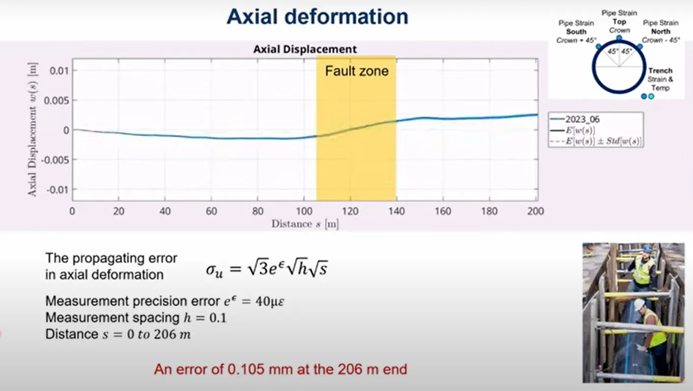
He continued: “Distributed strain data can be integrated along the axial direction to get the relative displacement profile from one end of the pipe to other end in terms of stretching of the pipe.”
Seasonal variations were observed – with slight compression occurring in winter and minor extension in summer due to the thermal contraction and expansion of the plastic pipe.
“However, such thermal induced axial movement is constrained by soil resistance in the axial direction,” he added. “On the other hand, the axial extension around the area of the fault zone is about 4mm, and this is due to the localised strain accumulation over the region.
“As the distributed strain are integrated, errors accumulate as you integrate over distance. A theoretical formula can be derived to quantify this accumulation as shown [in the below] equation. The error originates from the precision error, as well as the measurement spacing […] and the integration distance. The estimation indicates the error at the 206m end point is approximately 0.1mm, which is relatively small compared to the 4mm that we measured.
“The 4mm elongation observed around the fault line over the 18 months can be compared with the data from the interferometric synthetic aperture radar (InSAR), which has been collected over more than 10 years. Although InSAR data exhibits significant scatter, it statistically shows that relative movement between the Pacific Plate and the Northern American Plate with a displacement rate of approximately 4mm per year. So this aligns well with the estimate derived from the DFOS measurements.”
The two fibre optic cables on the two sides of the pipeline provide data sets to derive the bending strain, which can then provide the lateral displacement of the pipeline.
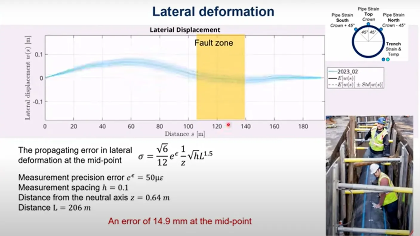
The results showed “surprising” lateral movement of approximately 100mm.
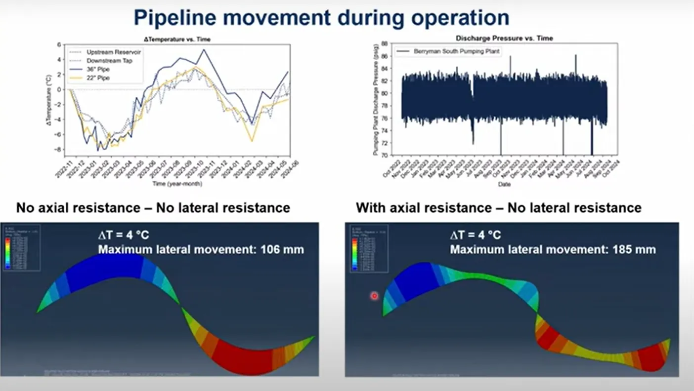
“Area estimates indicate uncertainty of about 15mm at the midpoint, which is smaller than what we measured, which is 100mm. So, at the beginning when I saw this, it was hard to believe. However, it was observed that the temperature of the water inside the pipeline varies both daily and seasonally. Also, internal pressure fluctuates throughout the day as the water pumps to the reservoir and is then released for distribution.
“Plastic pipe has a large thermal expansion coefficient. A simplified soil spring interaction analysis was conducted to examine the effect of temperature and internal pressure variation on the pipe movement. When the later soil spring was assigned to be minimal resistant, thermal expansion and contraction of the pipeline allowed lateral movement similar to what was estimated from the fibre optic sensors.”
In addition, the trench was narrow and it was “unlikely that proper soil compaction was not achieved around the pipe”.
“However, where the location of maximum lateral movement occurred depends on actual resistance of the soil. When there’s no actual resistance, which is not likely, the maximum location is shown where the curvature is maximum. When there’s some actual resistance, the maximum location shifted, as shown in the [below] right figure.
“More work is needed to develop a predictive model, but the key takeaway is that daily and seasonal variation must be thoroughly understood before assessing effects of fault movement on pipeline displacements.”
Soga continued: “Monitoring with DFOS enables evaluation of anticipated performance, not only for a few points, but continuously along the entire asset. So, in this context, it is essential to know the variation in distributed strain profiles predicted by different models to assess how well they align with the observed performance.”
One key insight from the case study is the value of embedding “intelligent” sensing systems during pipeline installation, as once it is buried, it will remain there for the next 100 years.
“In this case study the monitoring data provided valuable insights into deformation mechanism of the HDPE pipeline, particularly in response to daily and seasonal temperature variations inside the pipeline,” Soga summarised.
“Understanding these strain fluctuations during normal operation enables better understanding and better preparation for potential strain changes caused by large fault movements during an earthquake.
“The pipeline is designed to withstand large ground movement after a large earthquake, but the strain sensors will allow for assessment of its residual life, informing future renewal decisions.”
DFOS can thus be adopted for proactive maintenance to ensure economic efficiency and long-term safety.
Conclusions
Soga concluded his lecture by summarising the key message of this talk – using the concept of a 50/50 prediction approach to monitor the performance of geotechnical infrastructure.
By using this approach, Soga said, you can begin to understand what the “50/50 threshold is for various uncertainties that need to be considered”.
“So, rather than just going for red, let’s try to find our 50/50,” he noted.
“The engineering assessment can start with predicted performance using both most probable and cautious parameters. Monitoring can then be conducted to evaluate where the collected data falls within the various categories of green, amber or red. When multiple readings are obtained during construction or from nearby sites, decision parameters can be refined through back analysis, which represents the learning stage. We can continue this cycle until we’re confident about 50/50.”
Soga ended the lecture with the following points:
Innovation in sensors and data analytics offer exciting opportunities in geotechnical engineering to understand the actual performance of infrastructure during both construction and operation. For instance, embedded distributed fibre optics can provide valuable strain data that no other sensors can offer.A monitoring system should be integral to the construction package. This ensures long-term proactive operational monitoring, contributing to quality control, maintenance, resilience against hazards, and reuse.The new generation observational method is a proactive integration of design calculations and monitoring: use of cautious parameters and most probable parameters; acquire knowledge from the monitoring data and appreciate different uncertainties; enhance economic efficiency and ensure future sustainability.
Watch the full lecture here.