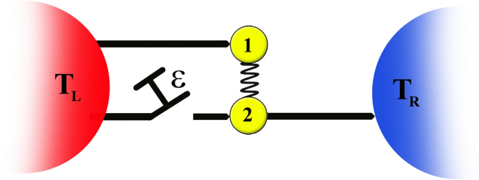
We now present numerical results for the dynamics of entanglement and heat current between the qubits for various initial two-qubit states in both the symmetric qubit-bath \((\varepsilon =0)\) and asymmetric qubit-bath \((\varepsilon =1)\) configurations. More importantly, we reveal the role of non-equilibrium effects on generation and protection of entanglement, in both the \(\varepsilon =0\) and \(\varepsilon =1\) cases, by investigating the effect of the temperature gradient of baths \(\Delta T=T_L-T_R\) on the dynamics of entanglement. Furthermore, we investigate heat current and the intriguing phenomenon of thermal rectification with emphasis on the role of asymmetry in the system-bath couplings.
Entanglement generation
In Fig. 3, we display dynamically generation of entanglement for the separable two-qubit initial state \(|\Phi _1\rangle =|00\rangle\), considering various values of the
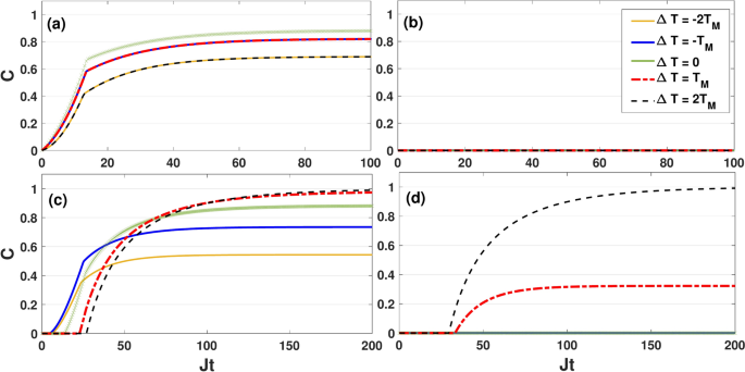
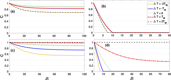
Dynamics of concurrence as a function of the dimensionless quantity Jt for different values of \(T_M\) by setting \(\kappa =0.05J\), \(B_0=0.6 J\) and \(\Delta =0.5 J\). The initial state is \(|\Phi _1\rangle =|00\rangle\). The plots correspond to the symmetric coupling configuration, i.e., \(\varepsilon =0\) (panels (a) and (b)) and asymmetric coupling configuration, i.e., \(\varepsilon =1\) (panels (c) and (d)). Panels (a) and (c), refer to \(T_M=0.5J\), while panels (b) and (d) refer to \(T_M=2J\).
temperature gradient \(\Delta T=T_L-T_R\). Here, we plot the concurrence as a function of Jt with the system parameters \(\kappa =0.05J\), \(\Delta =0.5J\) and \(B_0=0.6J\). In panels (a) and (b), the coupling switch is off \((\varepsilon =0)\) and thus the qubits interact with baths in the symmetrical coupling configuration, while in panels (c) and (d) the coupling switch is on \((\varepsilon =1)\) and thus the qubits interact with baths in the asymmetrical coupling configuration. Additionally, in panels (a) and (c) the mean temperature of the baths \(T_M=\frac{T_L+T_R}{2}\) is assumed to be low (e.g., \(T_M=0.5J\)), while in panels (b) and (d) \(T_M\) it is assumed to be sufficiently high (e.g., \(T_M=2J\)). We note that for initial state \(|\Phi _1\rangle =|00\rangle\), the coherence elements of matrix density \(\rho _{ij}(t)\) are zero, and therefore the Lamb shift does not affect the dynamical generation of entanglement between the qubits. Figure 3 shows that, at the low mean temperatures, the qubits become dynamically entangled in both the symmetric and asymmetric coupling configurations. Nevertheless, dynamically generation of qubit-qubit entanglement is possible only in the asymmetric coupling scenario when the mean temperature of baths is high enough (e.g., \(T_M=2J\) in the figures). Interestingly, in the asymmetric scenario, if entanglement is generated between the qubits, this occurs after a finite time has elapsed, whereas in the asymmetric scenario the qubits may become entangled at low mean temperature as soon as the dynamics begins.
To understand why the dynamical generation of qubit-qubit entanglement is possible in the asymmetric coupling configuration even when the mean temperature of baths is high enough, we look at the dynamics of the eigenstates populations \(\rho _{ii}=\langle \Phi _i|\rho |\Phi _i\rangle\) at high mean temperatures of the reservoirs. In Fig. 4 we plot \(\rho _{ii}\) as a function of the dimensionless quantity Jt for the initial state \(|\Phi _1\rangle\) corresponding to the panel (d) of Fig. 3.
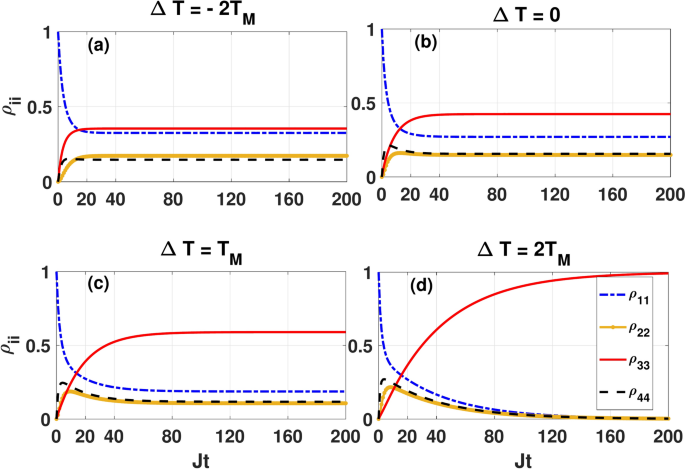
Dynamics of the eigenstates populations as a functions of the dimensionless quantity Jt for different values of \(\Delta T\) by setting \(\kappa =0.05J\), \(B_0=0.6 J\), \(\Delta =0.5 J\) and \(T_M=2J\). The plots correspond to the asymmetric coupling configuration (\(\varepsilon =1\)), and the initial state is \(|\Phi _1\rangle =|00\rangle\).
As one can see, due to the direct and indirect transitions from \(|\Phi _1\rangle\) to \(|\Phi _2\rangle\), \(|\Phi _3\rangle\) and \(|\Phi _4\rangle\), the eigenstate populations \(\rho _{11}\) (\(\rho _{jj}\), \((j=2,3,4)\)) decreases (increase) with time and then approaches some steady-state values depending on the value of \(\Delta T\). Also, at equilibrium condition at which the steady state of the system obeys the Gibbs distribution, the steady-state populations satisfy the ordering \(\rho _{22} as expected because the eigenstates satisfy the ordering \(E_3 for \(B_0\le |J+\Delta |\). When the positive temperature gradient increases, the steady-state populations of \(|\Phi _1\rangle\), \(|\Phi _2\rangle\) and \(|\Phi _4\rangle\) decreases, leading to an increase in the steady-state population of the ground state \(|\Phi _3\rangle\). Specially, at the higher temperature gradient \(\Delta T=2T_M\), once the system reaches the steady state, it populates exactly at the Bell state \(\Phi _3\) which is sufficient for the two-qubit steady-state concurrence to reach its maximum value. The physical reason behind the dynamical behavior of the populations at higher temperature gradient \(\Delta T=2T_M\) is quite clear: As we saw in the previous section, the transitions \(|\Phi _3\rangle \leftrightarrow |\Phi _1\rangle\) and \(|\Phi _3\rangle \leftrightarrow |\Phi _2\rangle\), induced by the interaction of the system with the left bath are never allowed in the asymmetric coupling configuration. On the other hand, from Eq. (12a), fixing \(T_L\) and
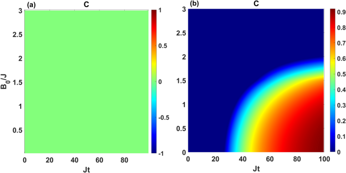
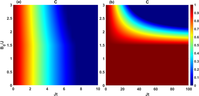
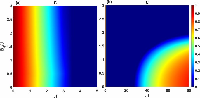
Dynamics of concurrence as a function of the dimensionless quantity Jt and magnetic field \(B_0/J\) for the initial state \(|\Phi _1\rangle =|00\rangle\) by setting \(\kappa =0.05J\), \(T_M=2J\), \(\Delta T=2T_M\) and \(\Delta =0.5 J\). The panels (a) and (b) correspond to the symmetric coupling setting, i.e., \(\varepsilon =0\) and asymmetric coupling setting, i.e., \(\varepsilon =1\), respectively.
taking the limit \(T_R\simeq 0\) (the high temperature gradient limit), we have \(\gamma _{13}^{(R,a)}=\gamma _{23}^{(R,a)}=0\), \(\gamma _{13}^{(R,e)}=\frac{\kappa (J+\Delta -B_0)}{2}\) and \(\gamma _{23}^{(R,e)}=\frac{\kappa (J+\Delta +B_0)}{2}\) for \(B_0\le |J+\Delta |\). This means that at high temperature gradients and for \(B_0\le |J+\Delta |\), the transitions from the entangled two-qubit Bell state \(|\Phi _3\rangle\) into the separable basis \(|\Phi _1\rangle\) and \(|\Phi _2\rangle\) induced by the interaction of qubits with the right bath are forbidden, but the reverse transitions occur. Therefore, in the asymmetric coupling configuration, the population of the Bell state \(|\Phi _3\rangle\) always increases at \(\Delta T=2T_M\) and for \(B_0\le J+\Delta\), leading to a population trapping phenomenon90 in this temperature gradient limi.
In Fig. 5 we investigate the effect of magnetic field \(B_0\) on the dynamically generation of entanglement between the qubits \(|\Phi _1\rangle =|0,0\rangle\). We here plot the concurrence as a function of \(\tau =J t\) and \(B_0/J\) for the mean temperature \(T_M=2J\) by adjusting the system parameters as \(\kappa =0.05J\), \(\Delta =0.5J\), and \(\Delta T=2T_M\). Panel (a) depicts the dynamics of concurrence in the symmetric configuration, while panel (b) corresponds to the asymmetric coupling configuration. It is evident that the generation of entanglement is not affected by the magnetic field when the coupling switch is flipped off (\(\varepsilon =0\)). However, when the coupling switch is on (\(\varepsilon =1\)), the generated entanglement at the long times decreases with the magnetic field, as shown in panel (b).
Entanglement protection
In Fig. 6, we display the dynamics of entanglement for the initial maximally entangled state \(|\Phi _3\rangle =\frac{1}{\sqrt{2}}\left[ |0,1\rangle -|1,0\rangle \right]\), corresponding to the panels of Fig. 3. We note that for the chosen initial state, the coherence elements of matrix density \(\rho _{ij}(t)\) become zero, and therefore the Lamb shift does not affect the dynamics of entanglement.
Dynamics of concurrence as a function of the dimensionless quantity Jt for different values of \(T_M\) by setting \(\kappa =0.05J\), \(B_0=0.6J\) and \(\Delta =0.5 J\). The initial state is \(|\Phi _3\rangle =\frac{1}{\sqrt{2}}\left[ |0,1\rangle -|1,0\rangle \right]\). The plots correspond to the symmetric coupling setting \((\varepsilon =0)\) (panels (a) and (b)) and asymmetric coupling setting \((\varepsilon =1)\) (panels (c) and (d)). Panels (a) and (c), refer to \(T_M=0.5J\), while panels (b) and (d) refer to \(T_M=2J\).
In the symmetric scenario, as shown in Fig. 6a,b, concurrence starts from its maximum value, decays over time and finally reaches a nonzero steady-state value for the chosen temperature gradient \(\Delta T\). We find that increasing the temperature gradient speeds up the decay rate of concurrence in both the low and high temperature regimes. This implies that the non-equilibrium feature of the environments plays a destructive role in protecting the initial entanglement of qubits in the symmetric coupling configuration. In the asymmetric coupling, however, increasing the temperature gradient, albeit at the positive bias, markedly slows down the decay rates of concurrence as illustrated in Fig. 6c,d. In particular, one could stop entanglement decay even at a high base temperature of the baths, provided the temperature gradient is increased to \(\Delta T=2T_M\). These results indicate that the temperature gradient between the reservoirs plays a constructive role in protecting the initial entanglement of qubits in the asymmetric coupling configuration.
To understand why in panels (c) and (d) the concurrence does not decay below one under the extreme condition (i.e., in the higher positive temperature gradient limit), we turn to previous subsection, where we proved that the transitions from the entangled two-qubit Bell state \(|\Phi _3\rangle\) into other eigenstates are forbidden in the higher positive temperature gradient limit \(\Delta T=2T_M\) for \(B_0\le J+\Delta\). Therefore, in Fig. 6 entanglement preservation can be the result of confining the dynamics to the decoherence-free subspace \(|\Phi _3\rangle\) of the system’s Hilbert space. Note that a decoherence-free subspace is a subspace of a quantum system’s Hilbert space that is invariant to non-unitary dynamics. The states belonging to this subspace are called sub-radiant states.
Dynamics of concurrence as a functions of the dimensionless quantity Jt and magnetic field \(B_0/J\) for the initial state \(|\Phi _3\rangle =\frac{1}{\sqrt{2}}\left[ |0,1\rangle -|1,0\rangle \right]\) by setting \(\kappa =0.05J\), \(T_M=2J\) and \(\Delta =0.5 J\). The panels (a) and (b) correspond to the symmetric coupling setting \((\varepsilon =0)\) and asymmetric coupling setting \((\varepsilon =1)\), respectively.
Furthermore, in Fig. 7 we have explored the effect of the magnetic field on the preservation of the initial entanglement contained in \(|\Phi _3\rangle\) when the base temperature of reservoirs is relatively high (e.g., for \(T_M=2J\)). The panels (a) and (b) display concurrence as a function of Jt and \(B_0/J\) in the symmetric and asymmetric coupling configurations, respectively. Here the system parameters are chosen as \(\kappa =0.05J\), \(\Delta =0.5J\), and \(\Delta T=2T_M\). According to panel (a), when the coupling switch is flipped off (\(\varepsilon =0\)), the dynamics of concurrence is almost insensitive to changes in the magnetic field strength. However, when the switch is flipped on (\(\varepsilon =1\)), the dynamics of concurrence can be controlled by the magnetic field, as shown in panels (b). We observe that the decay of concurrence is slowed down by decreasing the strength of the magnetic field, thereby completely protecting the initial maximal entanglement of the qubits by adjusting the strength of the magnetic field within interval [0, 1.5J].
Entanglement death and rebirth
Finally, we explore the dynamics of entanglement for the initial maximally entangled state \(|\Phi _4\rangle =\frac{1}{\sqrt{2}}\left[ |0,1\rangle +|1,0\rangle \right]\). Here the Lamb shift does not affect the dynamics of entanglement because of the chosen initial state.
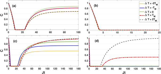
Dynamics of concurrence as a function of the dimensionless quantity Jt for different values of \(T_M\) by setting \(\kappa =0.05J\), \(B_0=0.6J\) and \(\Delta =0.5 J\). The initial state is \(|\Phi _4\rangle =\frac{1}{\sqrt{2}}\left[ |0,1\rangle +|1,0\rangle \right]\). The plots are related to the symmetric coupling setting \((\varepsilon =0)\) (panels (a) and (b)) and asymmetric coupling setting \((\varepsilon =1)\) (panels (c) and (d)). Panels (a), (c), refer to \(T_M=0.5J\), while panels (b), (d), refer to \(T_M=2J\).
In Fig. 8, we depict concurrence as a function of Jt for different values of \(\Delta T\), corresponding to the panels of Fig. 3. The results indicates that concurrence starts from its maximum value, dissipates to zero over the time (entanglement death), but rebirth after a period of time and finally reaches a steady-state value (entanglement rebirth). Comparing panels (a) with (b) and also (c) with (d) reveals that increasing the mean temperature \(T_M\) speeds up the death rate of entanglement in both symmetric and asymmetric coupling configurations. Notably, in the symmetric coupling configuration, high mean bath temperatures prevent the revival of dead entanglement. While, when entanglement death is followed by revival in the symmetric coupling configuration at low mean temperature, it occurs relatively quickly compared to the asymmetric coupling configuration.
Furthermore, similar to the dynamics of concurrence for the initial states \(|\Phi _1\rangle\) and \(|\Phi _3\rangle\), the non-equilibrium effect exhibits contrasting roles in the symmetric and asymmetric coupling configurations. In the symmetric coupling configuration, increasing temperature gradient suppresses the entanglement rebirth, as illustrated in panels (a) and (b), while in the asymmetric coupling configuration, the amount of revived entanglement enhances with the temperature gradient and becomes comparable to its initial maximum (see panels (c) and (d)). In the asymmetric configuration, a complete revival is achieved by adjusting the temperature gradient to \(\Delta T= 2T_M\). These findings imply that the non-equilibrium feature of the environments plays a destructive (constructive) role in reviving the initial entanglement of qubits in the symmetric (asymmetric) coupling configuration.
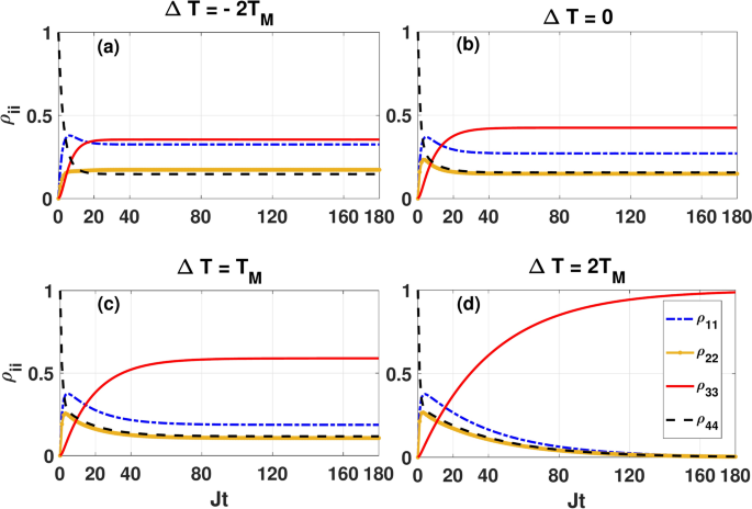
Dynamics of the eigenstates populations as a functions of the dimensionless quantity Jt for different values of \(\Delta T\) by setting \(\kappa =0.05J\), \(B_0=0.6 J\), \(\Delta =0.5 J\) and \(T_M=2J\). The plots correspond to the asymmetric coupling configuration (\(\varepsilon =1\)), and the initial state is \(|\Phi _4\rangle =\frac{1}{\sqrt{2}}\left[ |0,1\rangle +|1,0\rangle \right]\).
In order to gain a physical understanding of the behavior of concurrence in the asymmetric configuration, it is useful to explore dynamical behavior of the eigenstate populations for the initial state \(|\Phi _4\rangle\). In Fig. 9 we plot the eigenstate populations \(\rho _{ii}\) as a function of the dimensionless quantity Jt for the initial state \(|\Phi _4\rangle\) corresponding to panel (d) of Fig. 8. This figure shows that, as soon as the evolution starts, the direct transitions from \(|\Phi _4\rangle\) to \(|\Phi _1\rangle\) and \(|\Phi _2\rangle\) (please see Fig. 2) lead to a rapid increase in the population of the eigenstates \(|\Phi _1\rangle\) and \(|\Phi _2\rangle\), while the indirect transition between \(|\Phi _4\rangle\) and \(|\Phi _3\rangle\) leads to a slow increase in the population of \(|\Phi _3\rangle\). In turn, this suggests sudden death of entanglement at the beginning of the evolution. As can be seen, the population of \(|\Phi _3\rangle\) increases monotonously with time to reach its steady-state value. For \(\Delta T\le 0\), this increase is too small for the combined weight of the populations on the eigenstates to be able revive the dead entanglement. However, as illustrated in panels (c) and (d), for \(\Delta T>0\), the population of \(|\Phi _3\rangle\) increases over time and exceeds 0.5 which is sufficient to revive the dead qubit-qubit entanglement after a period of time. At higher temperature gradient \(\Delta T=2T_M\), the steady-state population of \(|\Phi _1\rangle\), \(|\Phi _2\rangle\) and \(|\Phi _4\rangle\) becomes zero and thus the system populates exactly at the Bell state \(|\Phi _3\rangle\). This explains why in Fig. 8 the lines for \(\Delta T=2T_M\) reach one at steady state, while those for other values of \(\Delta T\) do not.
In Fig. 10, we examine the effect of magnetic field on the entanglement dynamics of the initial state \(|\Phi _4\rangle\) when the base temperature of baths is relatively high. In this figure, the panels (a) ((b)) corresponds to dynamics of concurrence in the symmetric (asymmetric) configuration. From panel (a), it is evident that, similar to the entanglement dynamics of the initial states \(|\Phi _1\rangle\) and \(|\Phi _3\rangle\), the entanglement of the initial state \(|\Phi _4\rangle\) is not affected by the magnetic field when the coupling switch is off.
Dynamics of concurrence as a functions of the dimensionless quantity Jt and magnetic field \(B_0/J\) for the initial state \(|\Phi _4\rangle =\frac{1}{\sqrt{2}}\left[ |0,1\rangle +|1,0\rangle \right]\) by setting \(\kappa =0.05J\), \(T_M=2J\) and \(\Delta =0.5 J\). Panel (a) and (b) correspond to the symmetric coupling setting \((\varepsilon =0)\) and asymmetric coupling setting \((\varepsilon =1)\), respectively.
However, our results in panel (b) show that when the coupling switch is on, magnetic field affects the entanglement dynamics of \(|\Phi _4\rangle\). As shown in this panel, with the increase of \(B_0/J\) the revival time is shifted to longer times.
Heat current and thermal rectification: without the Lamb shift contribution
In this section we investigate the transient energy (heat) exchange between the qubits and reservoirs as well as thermal rectification, for the separable two-qubit initial states \(|\Phi _1\rangle =|00\rangle\) as well as the entangled two-qubit \(|\Phi _3\rangle =\frac{1}{\sqrt{2}}\left[ |0,1\rangle -|1,0\rangle \right]\) and \(|\Phi _4\rangle =\frac{1}{\sqrt{2}}\left[ |0,1\rangle +|1,0\rangle \right]\). Here, for simplicity, but without loss of generality, we ignore the Lamb shift contribution to the Lindblad equation (6).
In Fig. 11, we plot \(Q_L\) and \(Q_R\) as a function of Jt for different values of \(\Delta T\) in both symmetric and asymmetric coupling configurations. The system parameters are the same as in Fig. 3.
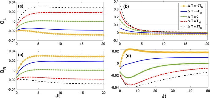
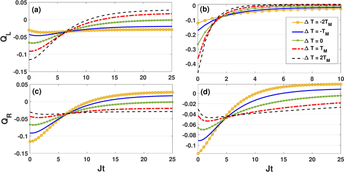
Dynamics of heat current \(Q_L\) and \(Q_R\) as a function of the dimensionless quantity Jt for different values of \(\Delta T\) by setting \(\kappa =0.05J\), \(B_0=0.6J\), \(\Delta =0.5 J\) and \(T_M=2J\). Here, the initial state of qubits is \(|\Phi _1\rangle =|00\rangle\) and the Lamb-shift term is not included. Panels (a) and (c) correspond to the symmetric coupling setting \((\varepsilon =0)\), while (b) and (d) correspond to asymmetric coupling setting \((\varepsilon =1)\) setting.
Panels (a) and (c) represent dynamics of quantum heat current in the symmetric coupling configuration, while (b) and (d) display dynamics of quantum heat current in the asymmetric coupling configuration. As expected, in both the symmetric and asymmetric coupling settings, the absolute value of the heat current increases with the temperature gradient. In the symmetric coupling scenario, as shown in the panels (a) and (c), heat initially flows from the qubits into the hot and cold bath. However, after some time, the direction of heat transfer from the qubits to the hot bath is reversed and the qubits start to absorb heat from the hot bath and reject it to the cold one. At this stage, the heat current absorbed (released) from (to) the hot (cold) bath increases with time to saturate at the steady-state values. In the symmetric coupling setting, the quantum heat currents \(Q_L\) and \(Q_R\) are equal regardless of the temperature gradient’s sign, as expected. However, the heat current seems to saturate faster (slower) by increasing \(\Delta T\) for the positive (negative) temperature gradient. In contrast, the dynamics of \(Q_L\) and \(Q_R\) undergo significant changes when coupling asymmetry is turned on, as depicted in panels (b) and (d).
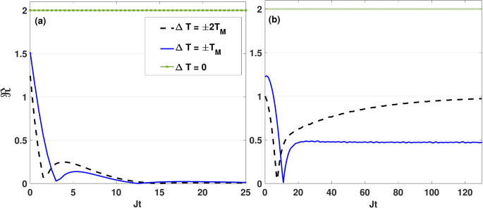
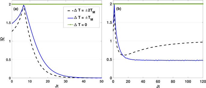
Dynamics of the thermal rectification factor \(\Re\) as a function of the dimensionless quantity Jt for different values of \(\Delta T\) by setting \(\kappa =0.05J\), \(B_0=0.6J\), \(\Delta =0.5 J\) and \(T_M=2J\). Here, the initial state of qubits is \(|\Phi _1\rangle =|00\rangle\) and the Lamb-shift term is not included. Panels (a) and (b) correspond to the symmetric coupling setting \((\varepsilon =0)\) and asymmetric coupling setting \((\varepsilon =1)\), respectively.
Here, \(Q_L\) consistently decreases over time, while \(Q_R\) initially increases to a maximum value before decaying to its steady-state value. Obviously, the saturation of heat currents occurs more slowly in the asymmetric coupling setting compared to the symmetric one. We find that, due to the additional connection between the qubit 2 and the hot bath, the transient heat current absorbed from the hot bath by the qubits is greater than the heat released to the cold bath. However, this situation alters in the steady-state limit, where the heat exchange with the hot source vanishes and the qubits release heat only to the cold bath.
In Fig. 12, we present the computed dynamical behavior of the thermal rectification factor for the initial state \(|\Phi _1\rangle\) in both the symmetric coupling (Fig. 12a) and asymmetric coupling (Fig. 12b) settings. The Lamb-shift corrections is not included here. Both Fig. 12a,b confirm that, at the equilibrium condition (\(\Delta T=0\)), heat flows through the qubits independent of the temperature gradient’s sign, resulting in \(\Re =2\). The thermal rectification factor \(\Re\) exhibits nonlinear characteristics under non-equilibrium conditions, which are consequences of the behavior of the heat current at each positive and negative temperature bias. In the symmetric coupling setting, \(\Re\) decays oscillatory to zero and a perfect rectification (\(\Re =1\)) is achieved at early times, as shown in Fig. 12a. In the asymmetric coupling setting, however, \(\Re\) experience different dynamics: it initially reaches a maximum, then decreases to near zero, before increasing again to attain a nonzero steady-state value. Therefore, the dynamics of the thermal rectification lasts longer in the asymmetric coupling setting in comparison to the symmetric coupling setting. Another positive aspect of the asymmetry in system-bath couplings is that both the steady-state rectification and the time required to reach the steady state increase with the magnitude of \(\Delta T\), enabling perfect rectification

Dynamics of heat current \(Q_L\) and \(Q_R\) as a function of the dimensionless quantity Jt for different values of \(\Delta T\) by setting \(\kappa =0.05J\), \(B_0=0.6J\), \(\Delta =0.5 J\) and \(T_M=2J\). Here, the initial state of qubits is \(|\Phi _3\rangle =\frac{1}{\sqrt{2}}\left[ |0,1\rangle -|1,0\rangle \right]\) and the Lamb-shift term is not included. The panels (a) and (c) correspond to the symmetric coupling setting \((\varepsilon =0)\), while (b) and (d) correspond to asymmetric coupling setting \((\varepsilon =1)\) setting.
when \(\Delta T\) reaches its maximum value.
In Fig. 13, we plot dynamics of \(Q_L\) and \(Q_R\) as a function of Jt for the initial state \(|\Phi _3\rangle =\frac{1}{\sqrt{2}}\left[ |0,1\rangle -|1,0\rangle \right]\), corresponding to the panels of Fig. 11. Based on this figure, the initial state \(|\Phi _3\rangle\) results in totally different heat current dynamics. In the symmetric coupling setting, both heat currents \(Q_L\) and \(Q_R\) experience a decaying dynamics to saturate at the steady-state values at each positive and negative temperature bias. In this setting, the heat current received from the hot bath saturates slower (faster) by increasing \(\Delta T\) at the positive (negative) bias. As shown in the panels (a) and (c), the heat flows from the reservoirs to the qubits in the beginning of the evolution, but after a time, the direction of heat transfer from the cold bath to the qubits is reversed and the qubits start to transfer the heat from the hot bath to the cold one. Then, the heat current absorbed (released) from (to) the hot (cold) reservoir increases with time to saturate at the steady-state values. This phenomena is also observed in the asymmetric coupling setting but only for the left bath (see Fig. 13b,d): for \(\Delta T=-T_M\), \(Q_L\) increases with time and reaches a positive maximum value, then decays to saturate at a negative steady-state value. The drawn curves in panels (b) and (d) also show that in the asymmetric coupling setting qubits always absorb heat from the right reservoir for both the positive and negative temperature biases. For temperature gradients \(\Delta T\le 0\), \(Q_L\) increases with time and reaches a maximum value, then decays to saturate at the steady-state values. Obviously, the saturation of heat currents occurs more slowly than in the symmetric coupling setting. As we can see, for the case \(\Delta T= 2T_M\), the qubits never exchange heat with the reservoirs. The physical reason behind this effect is the following: In “Entanglement protection” we proved that in the limit \(T_R\simeq 0\) (\(\Delta T\rightarrow 2T_M\)) and in the regime in which we work (\(B_0\le J+\Delta\)), when the coupling switch is turned on (\(\varepsilon =1\)), the initial state \(|\Phi _3\rangle\) remains immune to dissipation, causing the population components \(\rho _{11}\), \(\rho _{22}\) and \(\rho _{44}\) remain zero at all times.
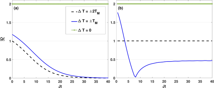
Dynamics of the thermal rectification factor \(\Re\) as a function of the dimensionless quantity Jt for different values of \(\Delta T\) by setting \(\kappa =0.05J\), \(B_0=0.6J\), \(\Delta =0.5 J\) and \(T_M=2J\). Here, the initial state of qubits is \(|\Phi _3\rangle =\frac{1}{\sqrt{2}}\left[ |0,1\rangle -|1,0\rangle \right]\) and the Lamb-shift term is included. The panels (a) and (b) correspond to the symmetric coupling setting \((\varepsilon =0)\) and asymmetric coupling setting \((\varepsilon =1)\), respectively.
On the other hand, adjusting \(\varepsilon =1\), and taking the limit as \(T_R\simeq 0\) (\(\Delta T\rightarrow 2T_M\)) in Eq. (12a), results in \(\gamma _{13}^{(R,a)}=\gamma _{13}^{(L,a)}=\gamma _{23}^{(R,a)}=\gamma _{23}^{(L,a)}=0\). By taking into account these considerations, it is straightforward from Eq. (23) that in the asymmetric coupling configuration, for \(\Delta T= 2T_M\), the heat current of the initial state \(|\Phi _3\rangle\) remains zero at all times.
In Fig. 14, we display the dynamics of the thermal rectification factor for the initial state \(|\Phi _3\rangle\) in both the symmetric coupling (Fig. 14a) and asymmetric coupling (Fig. 14b) settings. Both Fig. 14a,b reaffirm that, at equilibrium condition (\(\Delta T=0\)), heat flows through the qubits, independent of the sign of the temperature gradient, resulting in \(\Re =2\). In the symmetric coupling setting, as shown in Fig. 14a, \(\Re\) shows a monotonic decaying trend: for a given \(\Delta T\), the qubits acts as a thermal rectifier in the beginning of the evolution. After a time, when \(\Re\) decays monotonically to one, the qubits completely block the heat flow in one direction and thus behave as a perfect insulator. Then, as time goes on, the thermal rectification property of qubits gradually weakens again and finally disappears. As can be seen, when the temperature gradient increases to its maximum value, i.e. \(\Delta T=\pm 2T_M\), the qubits completely block the heat flow in one direction at the beginning of the evolution. However, they gradually lose their thermal rectification property over time until the heat flows symmetrically through the qubits.
In the asymmetric coupling setting, however, \(\Re\) follows a different dynamical pattern. In this setting, as illustrated in Fig. 14b,
Dynamics of heat current \(Q_L\) and \(Q_R\) as a function of the dimensionless quantity Jt for different values of \(\Delta T\) by setting \(\kappa =0.05J\), \(B=0.6J\), \(\Delta =0.5 J\) and \(T_M=2J\). Here, the initial state of qubits is \(|\Phi _4\rangle =\frac{1}{\sqrt{2}}\left[ |0,1\rangle +|1,0\rangle \right]\) and the Lamb-shift term is included. The panels (a) and (c) correspond to the symmetric coupling setting \((\varepsilon =0)\), while (b) and (d) correspond to the asymmetric coupling setting \((\varepsilon =1)\) setting.
the qubits completely lose their rectification property over time, but immediately regain it until the steady-state is reached. An interesting effect of this asymmetric coupling setting is observed at \(\Delta T=\pm 2T_M\), where the the heat flow is always completely blocked in one direction by the qubits, thus enabling the implementation of a stable thermal diode. In Fig. 15, we plot the dynamics of \(Q_L\) and \(Q_R\) as a function of Jt for the initial state \(|\Phi _4\rangle =\frac{1}{\sqrt{2}}\left[ |0,1\rangle +|1,0\rangle \right]\) in both the symmetric coupling [panels (a) and (c)] and asymmetric coupling [panel (b) and (d)] settings. According to the drawn curves, dynamics of the heat current in the symmetric coupling setting is almost the same as the dynamics in the asymmetric coupling setting. In both symmetric and asymmetric coupling settings, in general, the heat flows from the qubits to the reservoirs in the beginning of the evolution. However, after a certain time, the direction of heat transfer from the qubits to the hot bath is reversed and the qubits start to transfer the heat from the hot bath to the cold one. At this time, the heat current absorbed (released) from (to) the hot (cold) bath increases with time to saturate at the steady-state values. According to the drawn curves, the heat current received from the hot bath saturates slower by increasing \(\Delta T\). Similar to what can be seen for the initial states \(|\Phi _1\rangle\) and \(|\Phi _3\rangle\), the heat current received from the hot bath saturates more slowly (more quickly) as \(\Delta T\) increases at the positive (negative) bias.
Finally, in Fig. 16 we display the dynamics of the thermal rectification factor for the initial state \(|\Phi _4\rangle\) in both the symmetric coupling (Fig. 16a) and asymmetric coupling (Fig. 16b) settings. This figure again confirms that at the equilibrium condition (\(\Delta T=0\)),
Dynamics of the thermal rectification factor \(\Re\) as a function of the dimensionless quantity Jt for different values of \(\Delta T\) by setting \(\kappa =0.05J\), \(B=0.6J\), \(\Delta =0.5 J\) and \(T_M=2J\). Here, the initial state of qubits is \(|\Phi _4\rangle =\frac{1}{\sqrt{2}}\left[ |0,1\rangle +|1,0\rangle \right]\) and the Lamb-shift term is included. The panels (a) and (b) correspond to the symmetric coupling setting \((\varepsilon =0)\) and the asymmetric coupling setting \((\varepsilon =1)\), respectively.
the thermal rectification factor gets \(\Re =2\), indicating that, irrespective of the initial state of qubits, the heat flows through the qubits independent of the sign of the temperature gradient. In the symmetric coupling setting, for a given \(\Delta T\), the qubits rectify the heat in the beginning of the evolution. Then, when \(\Re\) suddenly increases to 2, the qubits transfer the received heat to the cold bath independent of the sign of the temperature gradient. After this time, the qubits start to rectify the heat again, completely blocking the heat flow in one direction once \(\Re\) decays to 1. Our results in Fig. 16a show that \(\Re\) eventually decays to zero at the steady state, indicating that qubits lose their rectification property upon reaching that state.
Furthermore, comparing Fig. 16a and b, it may be observed that dynamics of \(\Re\) in the asymmetric coupling setting is similar to the dynamics in the symmetric coupling setting, except in the steady-state limit where \(\Re\) has a nonzero value, indicating that the qubits exhibit thermal rectification. As can be seen, when the absolute temperature gradient increases to \(2T_M\), the steady-state rectification coefficient gets \(\Re =1\), where the qubits completely block the heat flow in one direction, thus realizing a thermal diode.
Before ending this section, we would like to comment on the relationship between the dynamical behavior of thermal entanglement and the phenomenon of heat rectification. By comparing Fig. 3 with 12, Fig. 6 with 14, and Fig. 8 with 16, one can clearly see that there is no a considerable relation between the dynamics of concurrence C and the dynamics of rectification coefficient \(\Re\). However, a close connection between rectification property and entanglement of qubits is observed in the asymmetric coupling setting when the system reaches the steady state. More precisely, for \(\varepsilon =1\), regardless of the initial state of qubits, both C and \(\Re\) reach one in the steady state when the gradient temperature of baths is \(\Delta T=2T_M\). This means that at the higher temperature gradient, qubits leverage the steady-state entanglement between themselves to completely block the heat released from the hot reservoir. This connection between thw steady-state rectification and steady-state entanglement can be explained as follows. As shown in Figs. 4d and 9d, at higher temperature gradient \(\Delta T=2T_M\) once the system reaches the steady-state, population of \(|\Phi _1\rangle\), \(|\Phi _2\rangle\) and \(|\Phi _4\rangle\) becomes zero and the system populates exactly at the maximally entangled state \(|\Phi _3\rangle\). This is while, if the temperatures of the left and right reservoirs are interchanged in the reverse direction, the populations \(|\Phi _1\rangle\), \(|\Phi _2\rangle\) and \(|\Phi _4\rangle\) will no longer be zero in the steady-state limit. On the other hand, in the asymmetric setting, we have \(\gamma _{13}^{(L,a)}=0\), \(\gamma _{13}^{(L,e)}=0\), \(\gamma _{23}^{(L,a)}=0\) and \(\gamma _{23}^{(L,e)}=0\), while \(\gamma _{ij}^{(\nu ,a)}\), \(\gamma _{ij}^{(\nu ,e)}\) \((i=1,2;j=3,4)\) are nonzero at \(\Delta T=-2T_M\). Therefore, according to Eq. (23), in the forward direction the heat current \(Q_L(\infty )\) becomes zero. However, in the reverse direction, while the mentioned absorption and emission rates remain zero, the populations of \(|\Phi _1\rangle\), \(|\Phi _2\rangle\), and \(|\Phi _4\rangle\) are no longer zero, resulting in \(Q_L^{r}(t)\ne 0\). This leads to the phenomenon of perfect rectification.
Lamb-shift contribution to the thermal rectification property of qubits
In the previous subsection, we have ignored the Lamb shift correction, i.e. the effective shift of the eigenenergies of the qubits induced by the presence of the baths. The effective shift of the eigenenergies depends on both mean temperature \(T_M\) and gradient temperature \(\Delta T\), thus it may influence the rectification properties of the qubits.
Dynamics of the thermal rectification factor \(\Re\) for different values of \(\Delta T\) with and without the Lamb shift. The initial state of the qubits is \(|\Phi _1\rangle =|0,0\rangle\) and other parameters are set as same as Fig. 12. In the presence of the Lamb shift, the cutoff frequency of the Ohmic spectral density is \(\omega _D=1000 J\). The panels (a) and (b) correspond to the symmetric coupling setting \((\varepsilon =0)\) and the asymmetric coupling setting \((\varepsilon =1)\), respectively.
As we now demonstrate, considering this correction allows us to achieve rectification dynamics different from that derived in the previous subsection. It is worth noting that for an Ohmic spectral density, the integrals that appear in Eq. (15) diverge. However, introducing a suitable cutoff frequency \(\omega _D\), resolves this divergence, yielding finite values for the integrals.
In Fig. 17, we illustrate the Lamb-shift contribution to the thermal rectification of the qubit for the initial state \(|\Phi _1\rangle\) in both the symmetric coupling (Fig. 17a) and asymmetric coupling (Fig. 17b) settings. Here, we plot the rectification factor \(\Re\) as a function of Jt for different values of \(\Delta T\) with and without the Lamb-shift in both symmetric and asymmetric coupling configurations. The system parameters are the same as in Fig. 3. Both Fig. 17a and b reveal that, at equilibrium condition (\(\Delta T=0\)), heat current among the qubits remains unaffected by the presence of the Lamb modification. We find that by taking into account the Lamb shift corrections, we attain rectification beyond the bounds derived in the previous sections. As shown in Fig. 17a, Lamb shift prevents qubits from achieving perfect rectification (\(\Re =1\)) in the symmetric setting. This implies that the bath-induced Lamb-shift correction plays a destructive role in the rectification performance of qubits in the symmetric coupling configuration. Conversely, Fig. 17b demonstrates that the Lamb-shift correction has a constructive effect in the asymmetric coupling configuration: for \(\Delta T=\pm T_M\), it increases the number of perfect rectification times and for \(\Delta T=2T_M\), it prolongs the perfect rectification time.
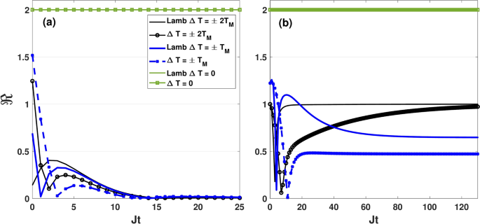
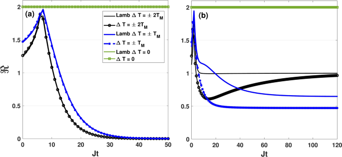
Dynamics of the thermal rectification factor \(\Re\) for different values of \(\Delta T\) with and without the Lamb shift. The initial state of qubits is \(|\Phi _3\rangle =\frac{1}{\sqrt{2}}\left[ |0,1\rangle -|1,0\rangle \right]\) and all other parameters are set as in Fig. 14. In the presence of the Lamb shift, the cutoff frequency of the Ohmic spectral density is \(\omega _D=1000 J\). The panels (a) and (b) correspond to the symmetric coupling setting \((\varepsilon =0)\) and the asymmetric coupling setting \((\varepsilon =1)\), respectively.
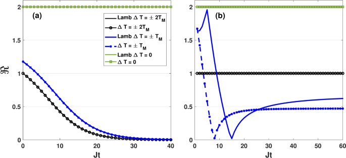
Dynamics of the thermal rectification factor \(\Re\) for different values of \(\Delta T\) with and without the Lamb shift. The initial state of qubits is \(|\Phi _4\rangle =\frac{1}{\sqrt{2}}\left[ |0,1\rangle +|1,0\rangle \right]\) and other parameters are set as same as Fig. 16. In the presence of the Lamb shift, the cutoff frequency of the Ohmic spectral density is \(\omega _D=1000 J\). The panels (a) and (b) correspond to the symmetric coupling setting \((\varepsilon =0)\) and the asymmetric coupling setting \((\varepsilon =1)\), respectively.
In Fig. 18, we illustrate Lamb-shift contribution to the thermal rectification of the qubits prepared in the initial state \(|\Phi _3\rangle\) in both the symmetric coupling (Fig. 18a) and asymmetric coupling (Fig. 18b) settings. Here, the system parameters are the same as in Fig. 14. We find that, unlike the symmetric coupling setting, the Lamb-shift correction can change dynamical behavior of rectification in the asymmetric coupling setting. For \(\Delta T=\pm T_M\), as can be seen in Fig. 18b, the Lamb-shift correction although decreases rectification effect of the qubits in the beginning of the evolution, but increases it after a long time. The drawn curves in Fig. 18b also indicate that the Lamb-shift correction does not affect rectification dynamics of the qubits when the gradient temperature is \(\Delta T=0\) and \(\Delta T=2T_M\).
Finally, in Fig. 19, we illustrate Lamb-shift contribution to the thermal rectification of qubit prepared in the initial state \(|\Phi _4\rangle\) in both the symmetric coupling (Fig. 19a) and asymmetric coupling (Fig. 19b) settings. Here, the system parameters are the same as in Fig. 16. According to Fig. 19, the dynamics of rectification is affected by the presence of the Lamb modification only in the asymmetric coupling setting. For \(\Delta T=2T_M\) the Lamb-shift correction prolongs the perfect rectification time, while for \(\Delta T=\pm T_M\) this correction enhances the steady-state rectification performance of the qubits.