In this section, we explain the significance of the fractional derivative and the working rule of the modified simple equation method to solve NLEEs.
M-fractional derivative
Fractional derivatives are essential in studying nonlinear evolution equations (NLEEs) because they model complex phenomena with greater precision than integer-order derivatives. They offer a flexible framework to capture the memory and hereditary properties inherent in many physical, biological, and engineering systems. By incorporating fractional derivatives, NLEEs can describe anomalous diffusion and wave propagation in heterogeneous media, resulting in more accurate predictions and solutions. This enhanced modeling capability is vital in fields such as viscoelasticity, fluid dynamics, and signal processing. Additionally, the use of fractional derivatives in NLEEs promotes the development of new analytical and numerical methods, improving the understanding and resolution of complex nonlinear problems. The increasing interest in fractional calculus highlights its importance in advancing both theoretical and applied research across various scientific disciplines, such as44,45,46,47,48,49,50. There are numerous fractional derivatives, including the Riemann-Liouville, Caputo, Atangana-Baleanu, conformable, and He’s fractal derivative, that have been extensively utilized in diverse contexts to characterize memory effects, hereditary features, and nonlocal behaviors in physical and engineering challenges47,48. In this study, we select the M-fractional derivative for its beneficial characteristics in addressing nonlinear evolution equations. This derivative is especially advantageous for maintaining the essential properties of the original equation while integrating fractional-order effects, rendering it appropriate for the analysis of soliton dynamics and wave propagation in intricate media. The M-fractional derivative provides versatility in mathematical expressions and preserves a balance between local and nonlocal characteristics, which is crucial for accurately representing realistic physical processes49,50. Consequently, the selection of the M-fractional derivative is warranted due to its capacity to yield more precise and physically significant solutions within the specified problem context.
Definition and some features of \(\:\varvec{M}\)-fractional derivative
Definition Given a function \(\:\phi\::[0,\infty\:)\to\:\left(-\infty\:,\:\infty\:\right)\), the \(\:M-\)fractional derivative is well-defined as follows:
$$\:{D}_{M,t}^{{\updelta\:},r}\underset{ϵ\to\:0}{{\varphi\:}_{r}\left(x\right)=\text{lim}}\frac{\phi\:\left(x\:{\varphi\:}_{r}\left(ϵ{x}^{-{\updelta\:}}\right)\right)-\phi\:\left(t\right)}{ϵ}\:,\:t>0,\:r>0.$$
Here, \(\:{\varphi\:}_{r}\left(x\right)\) is a single parameter truncated Mittag-Leffler function clear as51, and taking belongs to \(\:\left(\text{0,1}\right):\)
$$\:{\varphi\:}_{r}\left(x\right)=\sum\:_{n=0}^{k}\frac{{x}^{n}}{{\Gamma\:}(\varphi\:n+1)}$$
Modified simple equation method
In this subdivision, the procedure of the modified simple equation technique52,53 is explained step by step to solve fractional PDEs. Now, we consider the M fractional PDEs in the following form:
$$\:R\left({D}_{M,t}^{\mu\:,N}Q,{Q}_{x},{{D}_{M,t}^{\mu\:,N}Q}_{x},{Q}_{xx},{Q}_{xxx},\right)=0$$
(2)
Step i: We use the following wave transformation to convert Eq. (2) into Ode’s form.
$$\:{\upphi\:}={\beta\:}_{1}\text{x}-{\upomega\:}\frac{{\Gamma\:}\left(N+1\right)}{\mu\:}{t}^{\mu\:};\:\text{Q}\left(x,t\right)=Q\left({\upphi\:}\right)$$
(3)
Step ii: Insert Eq. (3) into Eq. (2).
$$\:R\left(-\omega\:{Q}_{{\upphi\:}},{\beta\:}_{1}{Q}_{{\upphi\:}},{-\omega\:{\beta\:}_{1}Q}_{{\upphi\:}{\upphi\:}},{\beta\:}_{1}^{2}{Q}_{{\upphi\:}{\upphi\:}},{\beta\:}_{1}^{3}{Q}_{{\upphi\:}{\upphi\:}{\upphi\:}},\right)=0$$
(4)
Step iii: The solution of Eq. (4) has the following form.
$$\:Q\left({\upphi\:}\right)=\sum\:_{q=0}^{s}\left({\alpha\:}_{q}{\left(\frac{H{\prime\:}\left({\upphi\:}\right)}{H\left({\upphi\:}\right)}\right)}^{q}\right)$$
(5)
Here \(\:{\alpha\:}_{s}\) is the unfamiliar constant. The balance number \(\:s\) can be derived from the following formula:
$$\:\frac{{d}^{p}Q}{d{{\upphi\:}}^{p}}=s+p\:\:\:and\:\:\:\:{Q}^{q}+{\left(\frac{{d}^{p}Q}{d{{\upphi\:}}^{p}}\right)}^{L}=qs+\text{L}\left(s+p\right)$$
Step iv: The trial solution Eq. (5) and its necessary form are submitted into Eq. (4). After calculation, we have a polynomial as: \(\:P\left(H\left({\upphi\:}\right)\right)={C}_{0}{\left(\frac{1}{H\left({\upphi\:}\right)}\right)}^{0}+{C}_{1}{\left(\frac{1}{H\left({\upphi\:}\right)}\right)}^{1}+{C}_{2}{\left(\frac{1}{H\left({\upphi\:}\right)}\right)}^{2}+{C}_{3}{\left(\frac{1}{H\left({\upphi\:}\right)}\right)}^{3}+,,,\), Now, we set \(\:{C}_{0}={C}_{1}={C}_{2}={C}_{3}=,,,,=0\). Now, using MAPLE 2023, the system of equations is solved for the values of \(\:{\alpha\:}_{q},\:\omega\:,{\beta\:}_{1},\:H\left({\upphi\:}\right)\). If we inject the obtained value of these parameters in Eq. (5), then the required values are obtained.
Bifurcation analysis
The time M-fGP-NWE equation is considered as:
$$\:{Q}_{\text{x}\text{x}\text{x}\text{y}}+{a}_{1}{D}_{M,t}^{\delta\:,r}{Q}_{\text{y}}+{a}_{2}{\left(\frac{{Q}^{n}}{n}\right)}_{xy}+{a}_{3}{Q}_{\text{x}\text{x}}+{a}_{4}{Q}_{\text{z}\text{z}}=0$$
(6)
To convert the Eq. (6) into ODE form, we apply the wave variable as
$$\:\text{Q}\left(x,y,z,t\right)=Q\left({\upphi\:}\right);\:{\upphi\:}={\beta\:}_{1}\text{x}+{\beta\:}_{2}\text{y}+{\beta\:}_{3}\text{z}-{\upomega\:}\frac{{\Gamma\:}\left(N+1\right)}{\delta\:}{t}^{\delta\:}$$
(7)
After inserting Eq. (7) into Eq. (6), the following ODE is obtained
$$\:{\beta\:}_{2}{\beta\:}_{1}^{3}{Q}_{{\upphi\:}{\upphi\:}{\upphi\:}{\upphi\:}}-{\upomega\:}{\beta\:}_{2}{a}_{1}{Q}_{{\upphi\:}{\upphi\:}}+{\beta\:}_{2}{\beta\:}_{1}{a}_{2}{\left(\frac{{Q}^{n}}{n}\right)}_{{\upphi\:}{\upphi\:}}+{\beta\:}_{1}^{2}{a}_{3}{Q}_{{\upphi\:}{\upphi\:}}+{\beta\:}_{3}^{2}{a}_{4}{Q}_{{\upphi\:}{\upphi\:}}=0$$
(8)
.
Integrating Eq. (8) with respect to \(\:{\upphi\:}\) and the following form obtained
$$\:{\beta\:}_{2}{\beta\:}_{1}^{3}{Q}_{{\upphi\:}{\upphi\:}}+{\beta\:}_{2}{\beta\:}_{1}{a}_{2}\frac{{Q}^{n}}{n}+\left({\beta\:}_{1}^{2}{a}_{3}+{\beta\:}_{3}^{2}{a}_{4}-{\upomega\:}{\beta\:}_{2}{a}_{1}\right)Q=0$$
(9)
Equation (9) develops as
$$\:{Q}_{{\upphi\:}{\upphi\:}}=\frac{-{\beta\:}_{2}{\beta\:}_{1}{a}_{2}{Q}^{n}+n\left({\upomega\:}{\beta\:}_{2}{a}_{1}-{\beta\:}_{1}^{2}{a}_{3}-{\beta\:}_{3}^{2}{a}_{4}\right)Q}{n{\beta\:}_{2}{\beta\:}_{1}^{3}}$$
(10)
Equation (10) develop as:
$$\:\left\{\begin{array}{c}\frac{dF}{d{\upxi\:}}=R\\\:\frac{dR}{d{\upphi\:}}=-{\lambda\:}_{1}{Q}^{\text{n}}+{\lambda\:}_{2}Q\end{array}\right.$$
(11)
where, \(\:{\lambda\:}_{1}=\frac{{a}_{2}}{n{\beta\:}_{1}^{2}},\:{\lambda\:}_{2}=\frac{\left({\upomega\:}{\beta\:}_{2}{a}_{1}-{\beta\:}_{1}^{2}{a}_{3}-{\beta\:}_{3}^{2}{a}_{4}\right)}{{\beta\:}_{2}{\beta\:}_{1}^{3}}\)
$$\:\mathcal{H}(Q,R)=\frac{{R}^{2}}{2}+\frac{{\lambda\:}_{1}{Q}^{\text{n}+1}}{\text{n}+1}-\frac{{\lambda\:}_{2}{Q}^{2}}{2}=h$$
(12)
In Eq. (12), the symbol \(\:h\) represents the Hamiltonian constant. From Eq. (11), the following systems are formulated.
$$\:\left\{\begin{array}{l}R=0,\\\:-{\lambda\:}_{1}{Q}^{\text{n}}+{\lambda\:}_{2}Q=0\end{array}\right.$$
(13)
By solving the System in Eq. (13), we get the following equilibrium points
$$\:{P}_{1}=\left(\text{0,0}\right),\:{P}_{2}=\left({\left(\frac{{\lambda\:}_{2}}{{\lambda\:}_{1}}\right)}^{\frac{1}{n-1}},0\right),\:{P}_{3}=\left(-{\left(\frac{{\lambda\:}_{2}}{{\lambda\:}_{1}}\right)}^{\frac{1}{n-1}},0\right)$$
From Eq. (13), we get,
$$\:j(Q,R)=\left|\begin{array}{cc}0&\:1\\\:-{\lambda\:}_{1}n{Q}^{\text{n}-1}+{\lambda\:}_{2}&\:0\end{array}\right|=-\left(-{\lambda\:}_{1}n{Q}^{\text{n}-1}+{\lambda\:}_{2}\right)$$
(14)
Based on Eq. (14), we make the following assumptions:
1.
If \(\:j\left({P}_{e}\right), then \(\:{P}_{e}\) becomes a saddle point
2.
If \(\:j\left({P}_{e}\right)>0\), then \(\:{P}_{e}\) becomes center point
3.
If \(\:j\left({P}_{e}\right)=0\), then \(\:{P}_{e}\) becomes cuspidor point
The results that can be obtained by adjusting the relevant parameter are outlined below:
$$\:\mathbf{C}\mathbf{a}\mathbf{s}\mathbf{e}\:1:\:{\lambda\:}_{1}>0\:\text{a}\text{n}\text{d}\:{\lambda\:}_{2}>0.$$
$$\:\text{W}\text{h}\text{e}\text{n}\:n=2,\:{\lambda\:}_{1}>0\:\text{a}\text{n}\text{d}\:{\lambda\:}_{2}>0,$$
There are two equilibrium points. At \(\:\left(\frac{{\lambda\:}_{2}}{{\lambda\:}_{1}},0\right)\), the all trajectories are closed, so the point \(\:\left(\frac{{\lambda\:}_{2}}{{\lambda\:}_{1}},0\right)\) is center point. At point \(\:\left(0,0\right)\), the all trajectories are not closed. So, the point \(\:\left(0,0\right)\) is saddle point in Fig. 1(a).
When \(\:n=3\)
There are three equilibrium points. At \(\:\left(-{\left(\frac{{\lambda\:}_{2}}{{\lambda\:}_{1}}\right)}^{\frac{1}{2}},0\right)\) and \(\:\left({\left(\frac{{\lambda\:}_{2}}{{\lambda\:}_{1}}\right)}^{\frac{1}{2}},0\right)\), the all trajectories are closed, so the points \(\:\left(-{\left(\frac{{\lambda\:}_{2}}{{\lambda\:}_{1}}\right)}^{\frac{1}{2}},0\right)\) and \(\:\left({\left(\frac{{\lambda\:}_{2}}{{\lambda\:}_{1}}\right)}^{\frac{1}{2}},0\right)\) are center point. At point \(\:\left(0,0\right)\), the all trajectories are not closed. So, the point \(\:\left(0,0\right)\) is saddle point in Fig. 1(b).
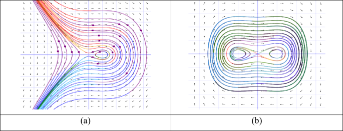
The two-dimensional phase diagram of the system Eq. (11) for the case \(\:{\lambda\:}_{1}>0\) and \(\:{\lambda\:}_{2}>0\).
$$\:\mathbf{C}\mathbf{a}\mathbf{s}\mathbf{e}\:2:\:{\lambda\:}_{1}0$$
$$\:\text{W}\text{h}\text{e}\text{n}\:n=2,\:{\lambda\:}_{1}0,$$
There are two equilibrium points. At \(\:\left(-\frac{{\lambda\:}_{2}}{{\lambda\:}_{1}},0\right)\), All the trajectories are closed, so the point \(\:\left(\frac{{\lambda\:}_{2}}{{\lambda\:}_{1}},0\right)\) is center point. At point \(\:\left(0,0\right)\). All the trajectories are not closed. So, the point \(\:\left(0,0\right)\) is the saddle point in Fig. 2(a).
$$\:\text{W}\text{h}\text{e}\text{n}\:n=3,\:{\lambda\:}_{1}0$$
There are one equilibrium points. At point \(\:\left(0,0\right)\), the all trajectories are not closed. So, the point \(\:\left(0,0\right)\) is saddle point in Fig. 2(b).
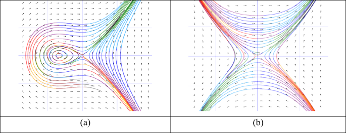
The two-dimensional phase diagram of the system Eq. (11) for the case \(\:{\lambda\:}_{1} and \(\:{\lambda\:}_{2}>0\).
$$\:\mathbf{C}\mathbf{a}\mathbf{s}\mathbf{e}\:3:\:{\lambda\:}_{1}>0\:\text{a}\text{n}\text{d}\:{\lambda\:}_{2}
$$\:\text{W}\text{h}\text{e}\text{n}\:n=2,\:{\lambda\:}_{1}>0\:\text{a}\text{n}\text{d}\:{\lambda\:}_{2}
There are two equilibrium points. At \(\:\left(-\frac{{\lambda\:}_{2}}{{\lambda\:}_{1}},0\right)\), All the trajectories are not closed, so the point \(\:\left(\frac{{\lambda\:}_{2}}{{\lambda\:}_{1}},0\right)\) is the saddle point. At point \(\:\left(0,0\right)\), All the trajectories are closed. So, the point \(\:\left(0,0\right)\) is the center point in Fig. 3(a).
$$\:\text{W}\text{h}\text{e}\text{n}\:n=3,\:{\lambda\:}_{1}>0\:\text{a}\text{n}\text{d}\:{\lambda\:}_{2}
There is one equilibrium point. At point \(\:\left(0,0\right)\), All the trajectories are closed. So, the point \(\:\left(0,0\right)\) is the center point in Fig. 3(b).
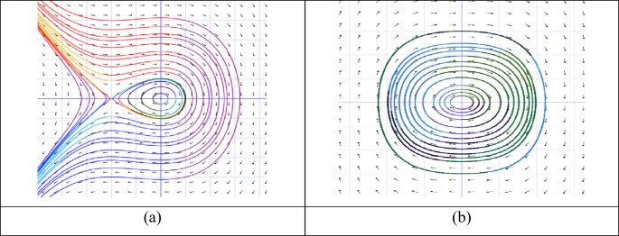
The two-dimensional phase diagram of the system Eq. (11) for the case\(\:\:{\lambda\:}_{1}>0\) and \(\:{\lambda\:}_{2}.
$$\:\mathbf{C}\mathbf{a}\mathbf{s}\mathbf{e}\:4:\:{\lambda\:}_{1}
$$\:\text{W}\text{h}\text{e}\text{n}\:n=2,\:{\lambda\:}_{1}
There are two equilibrium points. At \(\:\left(\frac{{\lambda\:}_{2}}{{\lambda\:}_{1}},0\right)\), all the trajectories are not closed, so the point \(\:\left(\frac{{\lambda\:}_{2}}{{\lambda\:}_{1}},0\right)\) is the saddle point. At point \(\:\left(0,0\right)\), all the trajectories are closed. So, the point \(\:\left(0,0\right)\) is the center point in Fig. 4(a)
$$\:\text{W}\text{h}\text{e}\text{n}\:n=3,\:{\lambda\:}_{1}
There are three equilibrium points. At \(\:\left(-{\left(\frac{{\lambda\:}_{2}}{{\lambda\:}_{1}}\right)}^{\frac{1}{2}},0\right)\) and \(\:\left({\left(\frac{{\lambda\:}_{2}}{{\lambda\:}_{1}}\right)}^{\frac{1}{2}},0\right)\), All the trajectories are not closed, so the points \(\:\left(-{\left(\frac{{\lambda\:}_{2}}{{\lambda\:}_{1}}\right)}^{\frac{1}{2}},0\right)\) and \(\:\left({\left(\frac{{\lambda\:}_{2}}{{\lambda\:}_{1}}\right)}^{\frac{1}{2}},0\right)\) are saddle points. At point \(\:\left(0,0\right)\), all the trajectories are closed. So, the point \(\:\left(0,0\right)\) is the center point in Fig. 4(b).
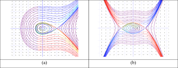
The two-dimensional phase diagram of the system Eq. (11) for the case \(\:{\lambda\:}_{1} and \(\:{\lambda\:}_{2}.