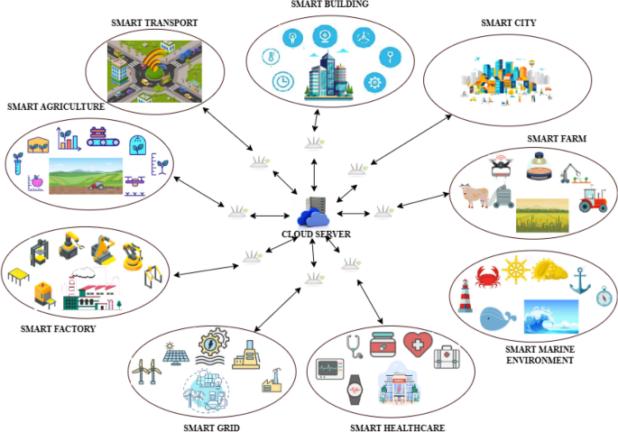
This section throws an insight into the various methods and techniques used in the proposed methodology for predicting the sensors’ battery life in an IoE environment. We highlight the ensemble base learner training technique and fusion methods, DL models used as base learners and the pre-processing methodology used for preparing the data.
Pre-processing methodologies
Data that is acquired from the real world is always messy with noise, missing values, errors and partial information. When the acquired data has to be used by ML, DL or EL models, the data has to be of high quality to land with highly accurate results. The pre-processing is the initial step in any AI-based model, which evaluates, filters, encodes and manipulates the acquired real-time data so that its quality is increased to be used by any AI model for learning44. The methodologies used in this proposed work for improving its quality are discussed in this subsection.
Label encoding scheme
When the acquired data consists of a wide range of numerical as well as categorical data, numerical data can be handled easily. But when the categorical data is in string or label format, then these cannot be processed directly by the AI model. The label encoding scheme is the process by which the string-based categorical data is converted into numerical data. In this scheme, every category in the data set is assigned a unique integer value. The major advantage of this scheme is that it does not increase the dimension of the data set. Also, it requires less computational time and resources when compared to other encoding schemes like one-hot encoding. This scheme is best suited for ordinal sets where a sequence or order has to be maintained in the category.
Standard scaler method
A standard scaler is a simple method that is based on the concept of normalization. Each feature is transformed in such a way that it has a mean of ‘0’ and a standard deviation of ’1’. This transformation is done to restrict any feature from dominating the learning process due to its large magnitude. The transformation is performed using the Eq. (8) below, where \(S_f\) represents the transformed value of the feature \(F_i\) for \(i=1,2,3,\ldots ,n\), \(\mu\) is the arithmetic mean and \(\sigma\) is the corresponding standard deviation.
$$\begin{aligned} S_f = F_i – \frac{\mu }{\sigma } \end{aligned}$$
(8)
This transformation step enhances the performance of the model, is robust towards the outliers and also helps in better interpretation ability.
Ensemble base learners
There are various types of Ensemble learning techniques which include Bagging, Boosting, Stacking and Blending. In the case of Bagging, the training data is sampled and each sample is trained with different base learners. The final prediction is the result of the averaging of individual predictions. Boosting is a technique that follows a sequential training pattern. The error that occurred in the first model is handled by the second model. The fusion method used in this case is usually the weighted average voting scheme. In the stacking technique, the prediction obtained from the first base model is given as input for the next-level model. The prediction result obtained from the higher-level model is considered to be the final prediction result.
Random forest regression
Random Forest Regression45 is a type of Ensemble Technique that is suitable for both classification and regression problems. In this type of Ensemble, multiple decision trees are built and the prediction results are combined to produce the final prediction result using both Bootstrapping and Aggregation methods. This is generally termed as Bagging. The Random Forest model is based on multiple decision trees (DT), and each DT is considered to be a base model. Each model is trained using different samples of the data set by using row sampling and feature sampling randomly. This step is called as Bootstrapping. Here the trees built run in parallel and do not have any interaction with each other. Random subsets are selected from the training set, and small decision trees are built. These smaller DTs are then combined to form the random forest model, which gives the final result. The graphical structure of the model is illustrated in Fig. 6a below. This helps in reducing the variance and increasing the accuracy. Random Forest Regression can be used in applications where there are continuous values like stock markets, sales, etc. This model is best suited for large data sets as it can capture the non-linear relationships among the input and target variables. The major advantages of using this model are less prone to over-fitting and can perform well when we have categorical variables and high dimensions. Some important features that motivate its usage are speed, accuracy, feature selection, automation, robustness, parallelization and stability.
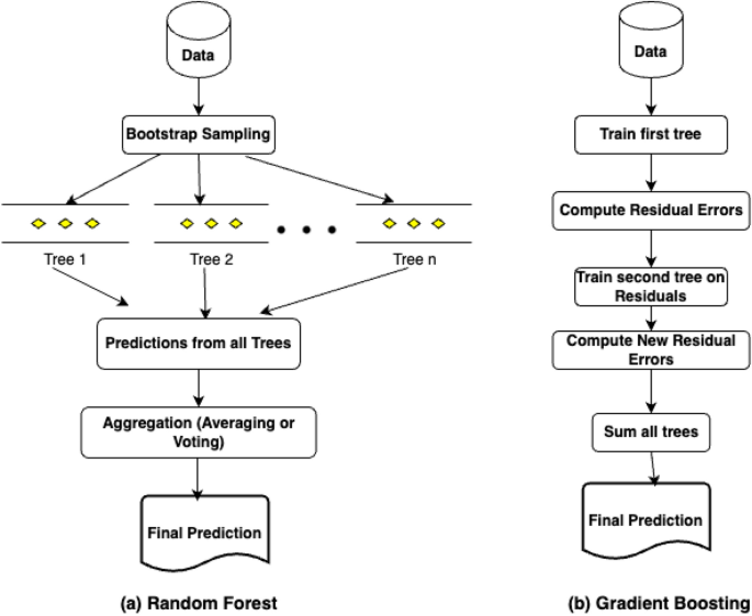
Graphical structure of random forest and gradient boosting regressor models.
Gradient boosting
Gradient Boosting is an Ensemble technique that can be used in all types of classification and regression tasks46. This is a kind of Boosting technique that tries to build the best model having less prediction error by merging all the earlier models. This technique is also referred to as statistical forecasting as it tries to eliminate the prediction errors of previous models. Based on the target, Gradient Boosting can be categorized into two types, namely Gradient Boosting Regressor and Gradient Boosting Classifier. Regressor is used when the target is continuous, whereas Classifier is used when the target is a classification variable. The Loss function plays a major role in differentiating these two variants. In the case of Regressor, the loss function can be anyone out of Mean Square Error, Mean Absolute Error and Huber. In the case of Classifier, the loss function can be either Deviance Loss or Exponential Loss. If there are total z samples and the target variable is represented as t, then the Mean Square Error (MSE) can be calculated using the Eq. (9). The graphical structure of the model is illustrated in Fig. 6b.
$$\begin{aligned} Mean Square Error = \frac{1}{z}\sum _{i=1}^{z}(t_i – t^*_i) \end{aligned}$$
(9)
where \(t_i\) is the actual target and \(t^*_i\) is the predicted target. Similarly, the Mean Absolute Error can be given by Eq. (10).
$$\begin{aligned} Mean Absolute Error = \frac{1}{z}\sum _{i=1}^{z}\left| t_i – t^*_i \right| \end{aligned}$$
(10)
The Deviance loss, which can also be referred to as Log loss or binary cross entropy loss, can be calculated using the Eq. (11). Here, \(p_i\) is the probability of prediction for Class \(C_n\) where n specifies the number of class labels in the classification problem.
$$\begin{aligned} Log Loss = -\frac{1}{z}\sum _{i=1, j=1}^{i=z, j=n}\left[ t_i log(p^*_i(C_n)) + (1-t_i)log(1-p^*_i(C_n)) \right] \end{aligned}$$
(11)
The Exponential Loss can be used in Boosting techniques like AdaBoost and can be represented as given in Eq. (12).
$$\begin{aligned} Exponential Loss = \frac{1}{z}\sum _{i=1}^{z}\exp (t_i – t^*_i) \end{aligned}$$
(12)
Categorical boosting
Categorical Boosting (CATBoost) is a type of Gradient Boosting mechanism that was developed by Yandex. This method can efficiently handle classification, regression and ranking tasks. They are best suited for categorical features. It is well known for its high speed and accuracy. The CatBoost algorithm functions using the oblivious trees instead of normal decision trees. In the case of oblivious trees, each node available at the same level uses similar splitting conditions concerning feature and threshold, as shown in the Fig. 7a. Also, unlike the other gradient boosting methods like Extreme Gradient Boosting and Light Gradient Boosting, this method can encode the categorical features automatically using ordered boosting and permutation-based encoding. Since ordered boosting is used for calculating the leaf values, over-fitting issues are handled. This also helps in preventing the target leakages. The method used for encoding is Categorical Target Statistics (CTR). Let us consider that the target categorical feature to be encoded is \(F^i_c,\) and the encoding is done using the Eq. (13) below.
$$\begin{aligned} CTR(F^i_c) = \frac{\sum _{j=1}^{n}y_j.I(F^j_c = F^i_c)}{\sum _{j=1}^{n}I(F^j_c = F^i_c)} \end{aligned}$$
(13)
where \(I(F^j_c = F^i_c)\) is an Indicator function whose value can be either 1 or 0 based on True or False values, respectively. In the fraction shown in Eq. (13), the numerator is the summation of the target values for which the indicator I is 1. The denominator represents the total number of such target occurrences. After this initial pre-processing step, the oblivious trees are constructed. Then, the gradient boosting process is carried out. The initial step here is to calculate the residuals using the Eq. (14) given below.
$$\begin{aligned} r_i = y – P_{i-1}(x) \end{aligned}$$
(14)
where \(r_i\) is the residual error at the ith iteration, y is the actual value and \(P_{i-1}(x)\) is the value predicted in the previous iteration. The model is then updated using the Eq. (15).
$$\begin{aligned} P_i(X) = P_{i-1}(x) + \rho . Tree_i(X) \end{aligned}$$
(15)
where \(\rho\) is the learning rate used.

Graphical structure of CatBoost and Light GBM models.
Light gradient boosting machine
Light Gradient Boosting Machine (LightGBM) is also a kind of gradient boosting framework that was developed by Microsoft. This is faster and more memory efficient when compared to other Gradient Boosting methods like XGB. The reason behind this is that LightGBM uses a special type of splitting called as histogram splitting. Also, the tree is constructed leaf-wise instead of level-wise, as shown in the Fig. 7b. The information gain of each leaf node is calculated, and the one with the maximum information gain is further split. This improves the efficiency of training since deeper and more optimized trees are generated within a few splits. The residual calculated in this method is called a pseudo-residual and is given by the Eq. (16)
$$\begin{aligned} r_i = \frac{\delta L(y, P_{i-1}(x))}{\delta P_{i-1}(x)} \end{aligned}$$
(16)
where \(L(y, P_{i-1}(x))\) is the Loss function, which may be RMSE or LogLoss, and \(P_{i-1}(x)\) is the prediction output of the previous iteration. RMSE is used in case of regression problems and LogLoss is used in classification problems. Using these residuals calculated, the Boosting step is carried out. Then histogram-based binning is performed for the features. Overfitting issues are handled by the L1 and L2 regularizations. Though there are advantages, this method is prone to overfitting due to the leaf-based deep tree construction. This is also not very suitable for small data sets.
Extreme gradient boosting regression
Extreme Gradient Boosting Regressor (XGBRegressor) is a modified version of Gradient Boosting Regressor, which can be implemented using various regulation techniques, including L1 and L2 regulation,the dropout method and early stopping. This method can reduce either over-fitting or under-fitting by reducing the value of the regulation coefficient47. The major advantage of this model is that it can perform pre-processing of each node in a parallel manner, hence saving time and landing with a faster prediction rate. XGB Machines can also automatically understand the imputations. When the complexity of the model goes high, regularization techniques like LASSO (L1) and Ridge (L2) are required to penalize it. The graphical structure is as shown in Fig. 8. The parameters required for regularization are as follows.
gamma (\(\gamma\)): This specifies the minimum reduction in loss allowed for the number of splits. When the value of gamma is high, then the number of splits is fewer and vice versa.
alpha (\(\alpha\)): This parameter is related to the L1 regularization and is on leaf weights. When this value is higher, there will be more regularization, which means that many leaf weights of the base learner are made zero.
lambda (\(\lambda\)): This parameter is related to the L2 regularization and provides a smooth decrease in leaf weights unlike L1 which has hard constraints.
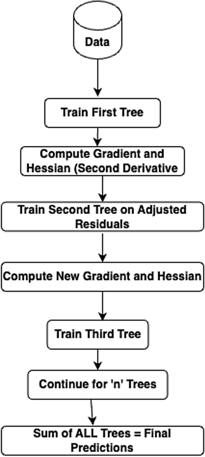
Graphical structure of extreme gradient boosting regression.
Multiple parameters help for building the trees in the regression, namely similarity score, gain, pruning criteria, etc. These parameters can be calculated as follows. In the Eq. (17), \(\rho\) represents the similarity score, \(r_i\) represents the residuals, and n represents the number of residuals. This parameter helps in growing the trees.
$$\begin{aligned} \rho = \frac{\sum _{i=1}^{n}r^2_i}{n} + \lambda \end{aligned}$$
(17)
For deciding on how to split the data, the parameter gain can be utilized and can be calculated by using the Eq. (18).
$$\begin{aligned} \eta = \rho _l + \rho _r – \rho _{root} \end{aligned}$$
(18)
where \(\eta\) is the gain, \(\rho _l\) is the similarity score of left tree, \(\rho _r\) is the similarity score of right tree and \(\rho _{root}\) is the similarity score of root. The tree is then pruned based on the value obtained using Eq. (14). If the value calculated is positive, then the tree is not pruned; if the result is negative, then the tree continues to be pruned further.
Linear regression
Linear Regression is a model that does the prediction by having an assumption that all variables are linked to each other under a straight-line relationship. Usually, the variables are considered to be independent and dependent. The relationship between these variables is calculated using a linear function. When the number of independent variables is one, then it is called as linear regression. The best fit straight line can be calculated using the Eq. (19), which is a traditional slope-intercept equation.
$$\begin{aligned} m_j = \beta _0 + \beta _1n_j \end{aligned}$$
(19)
where \(m_j\) is the dependent variable, \(n_j\) is the independent variable, \(\beta _0\) is the constant and \(\beta _1\) is the slope intercept. The performance of a Linear Regression model can be assessed using metrics like Coefficient of Determination (\(R^2\)), Root Mean Squared Error (RMSE) and Residual Standard Error (RSE). The Coefficient of Determination can be represented by Eq. (20), where \(R_s\) is the residual sum of squares and \(T_s\) is the total sum of squares.
$$\begin{aligned} R^2 = 1 – \frac{R_s}{T_s} \end{aligned}$$
(20)
The residual sum of squares can be calculated using Eq. (21), and the total sum of squares can be given by Eq. (22).
$$\begin{aligned} R_s= & \sum _{i=1}^{z}(m_j – \beta _0 – \beta _1n_j)^2 \end{aligned}$$
(21)
$$\begin{aligned} T_s= & \sum (m_j – m^*)^2 \end{aligned}$$
(22)
where \(m^*\) is the mean of all the data points j.
Stacking
Stacking is a powerful fusion method that combines the predictions of various base models to improve the performance of the final prediction. This is also called Stacked Generalization and is illustrated in Fig. 9. Stacking primarily focuses on providing the individual predictions of several base models or learners as input to the higher-level model termed “meta-model” or blender48. This meta-model finally combines or blends to provide a final prediction that is more accurate. Though traditional ensemble methods like bagging and boosting can be utilized, meta-learning provides a blended framework that leverages the advantages and performance of multiple models to produce an improved model. The meta-model learns to optimize the parameters and helps in generalization. This can also provide better model diversity. Meta-learning is best suited when the data sets are heterogeneous. Since we are focusing on developing a generalized framework for utilizing in the IoE environment, this is the best strategy to capture different complex aspects and relationships of the data. The steps involved in the procedure are data preparation, selection of model, training using the base models, prediction result on the validation data set, development of meta-model, training the meta-model, final predictions and evaluation of the model. Initially, the data set is prepared by cleaning and identifying the relevant features. Then, the entire data is subdivided into training and validation sets. Then, different models are selected to be used as base models for the ensemble approach. While selecting the models, various factors like diversity, hyper-parameters, type of errors, etc., are taken into account. Then the chosen base models are trained on the training set for learning the features. Once learning is complete, the validation data set is used for making predictions. Then, a meta-model is developed which is sometimes called a meta-learner that takes the predictions of the lower-level model as input and makes the final prediction. Any model like Linear Regression, Logistic Regression or Neural Network can be used for this purpose. The finalized meta-model is used for training the predictions obtained from the validation set. The initial predictions made by the base models are considered to be the features of the meta-model. The meta-model is then used for predicting the test set. Stacking generally produces an improved accuracy when compared to utilizing a single model.
Applying the above methodology, we performed experiments to test the predictive ability of our MetaStackD model. The following section describes the results, comparing model accuracy, efficiency, and relative performance with baseline models.