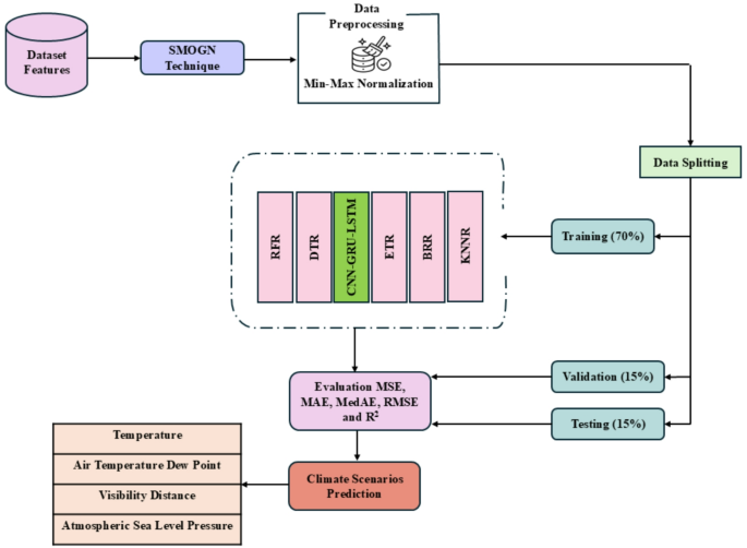
We conducted our experiments using Jupyter Notebook version 7.2.1, a popular tool for data analysis and visualization in Python. Jupyter Notebook offers a versatile environment for writing, running, and documenting code, as well as creating visual data representations. It supports various programming languages, including Python 3.10, and operates within a web browser. The experiments were run on a PC with Microsoft Windows 10, equipped with an Intel Core i7 CPU, 32GB of RAM, and an Nvidia RTX 2080 GPU. For developing and training our models, we used deep learning frameworks like TensorFlow and Keras. We also utilized several Python libraries, such as NumPy, Pandas, Matplotlib, and Scikit-learn, for data preprocessing, analysis, and visualization. In this study, we applied an advanced deep learning model known as the CNN-GRU-LSTM) to predict climate change in Al-Qassim Region, Saudi Arabia, up to 2050. The model evaluates 4 scenarios: temperature, air temperature dew point, visibility distance, and atmospheric sea level pressure. We compared the CNN-GRU-LSTM model’s performance with five traditional regression models: DTR, RFR, ETR, BRR, and KNNR. The performance was assessed using five metrics: MSE, MAE, MedAE, RMSE, and \(\:{(\text{R}}^{2})\). Table 3 shows the hyperparameter values for the machine learning regression models used in this study.
Table 4 presents the performance evaluation results for the CNN-GRU-LSTM model and five traditional machine learning regression models (DTR, RFR, ETR, BRR, and KNNR) in predicting the temperature, using evaluation metrics demonstrated in Eqs. (2–6). The CNN-GRU-LSTM model outperformed the other five regression models, achieving the lowest MSE, MAE, MedAE, RMSE and the highest \(\:{\text{R}}^{2}\) at 0.0102, 0.0805, 0.0676, 0.1010 and 99.62%, respectively. In contrast, the KNNR model outperformed the worst results, with higher values for MSE, MAE, MedAE, RMSE and lowest value for \(\:{\text{R}}^{2}\) at 0.0862, 0.7942, 0.4681, 0.2935 and 91.85%. The results of these metrics confirm the superior predictive performance of the proposed CNN-GRU-LSTM model compared to the other five traditional regression models.
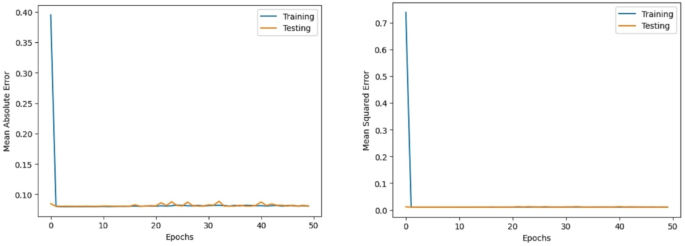
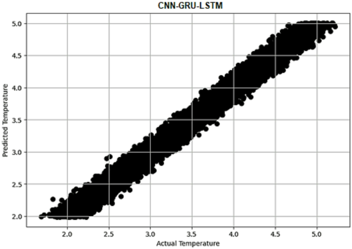
Figure 4 demonstrates the training and testing curves for mean squared error and mean absolute error vs. number of epochs using CNN-GRU-LSTM model for temperature prediction. It is clear from these curves that this model generalizes well from the acquired experience. Figure 5 depicts the actual temperature vs. predicted temperature using CNN-GRU-LSTM prediction model. It is clear from Fig. 5 that this model generalized unseen data reliably, indicating accurate prediction for temperature values.
Table 5 presents the performance evaluation results for the CNN-GRU-LSTM model and five traditional machine learning regression models (DTR, RFR, ETR, BRR, and KNNR) in predicting the air temperature dew point, using evaluation metrics demonstrated in Eqs. (2–6). The CNN-GRU-LSTM model outperformed the other five regression models, achieving the lowest MSE, MAE, MedAE, RMSE and the highest \(\:{\text{R}}^{2}\) at 0.0141, 0.0952, 0.0813, 0.1187 and 99.15%, respectively. In contrast, the KNNR model outperformed the worst results, with higher values for MSE, MAE, MedAE, RMSE and lowest value for \(\:{\text{R}}^{2}\) at 0.0984, 0.8403, 0.7582, 0.3136 and 91.27%. The results of these metrics confirm the superior predictive performance of the proposed CNN-GRU-LSTM model compared to the other five traditional regression models.
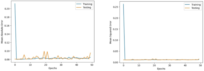
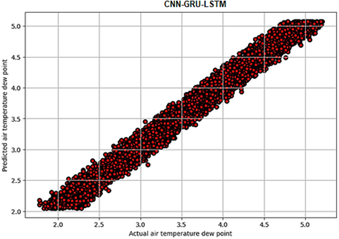
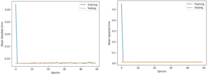
Figure 6 demonstrates the training and testing curves for mean squared error and mean absolute error vs. number of epochs using CNN-GRU-LSTM model for air temperature dew point prediction. It is clear from these curves that this model generalizes well from the acquired experience. Figure 7 depicts the actual air temperature dew point vs. predicted air temperature dew point using CNN-GRU-LSTM prediction model. It is clear from Fig. 7 that this model generalized unseen data reliably, indicating accurate prediction for air temperature dew point values.
Table 6 presents the performance evaluation results for the CNN-GRU-LSTM model and five traditional machine learning regression models (DTR, RFR, ETR, BRR, and KNNR) in predicting the visibility distance, using evaluation metrics demonstrated in Eqs. (2–6). The CNN-GRU-LSTM model outperformed the other five regression models, achieving the lowest MSE, MAE, MedAE, RMSE and the highest \(\:{\text{R}}^{2}\) at 0.0099, 0.0799, 0.0683, 0.0999 and 99.71%, respectively. In contrast, the KNNR model outperformed the worst results, with higher values for MSE, MAE, MedAE, RMSE and lowest value for \(\:{\text{R}}^{2}\) at 0.0951, 0.7594, 0.7251, 0.3083 and 90.73%. The results of these metrics confirm the superior predictive performance of the proposed CNN-GRU-LSTM model compared to the other five traditional regression models.
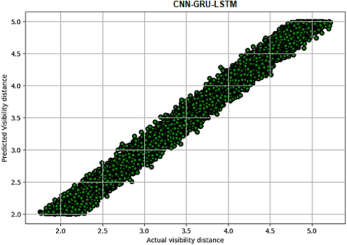
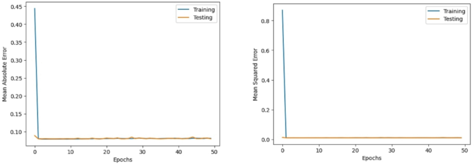
Figure 8 demonstrates the training and testing curves for MSE and MAE vs. number of epochs using CNN-GRU-LSTM model for visibility distance prediction. It is clear from these curves that this model generalizes well from the acquired experience. Figure 9 depicts the actual visibility distance vs. predicted visibility distance using CNN-GRU-LSTM prediction model. It is clear from Fig. 9 that this model generalized unseen data reliably, indicating accurate prediction for the visibility distance values.
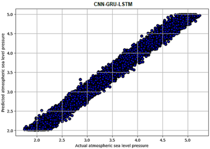
Table 7 presents the performance evaluation results for the CNN-GRU-LSTM model and five traditional machine learning regression models (DTR, RFR, ETR, BRR, and KNNR) in predicting atmospheric sea level pressure, using evaluation metrics demonstrated in Eqs. (2–6). The CNN-GRU-LSTM model outperformed the other five regression models, achieving the lowest MSE, MAE, MedAE, RMSE and the highest \(\:{\text{R}}^{2}\) at 0.0100, 0.0803, 0.0651, 0.1004 and 99.60%, respectively. In contrast, the KNNR model outperformed the worst results, with higher values for MSE, MAE, MedAE, RMSE and lowest value for \(\:{\text{R}}^{2}\) at 0.2758, 0.8072, 0.6475, 0.5251 and 90.02%. The results of these metrics confirm the superior predictive performance of the proposed CNN-GRU-LSTM model compared to the other five traditional regression models.
Figure 10 demonstrates the training and testing curves for mean squared error and mean absolute error vs. number of epochs using CNN-GRU-LSTM model for atmospheric sea level pressure prediction. It is clear from these curves that this model generalizes well from the acquired experience. Figure 11 depicts the actual atmospheric sea level pressure vs. predicted atmospheric sea level pressure using CNN-GRU-LSTM prediction model. It is clear from Fig. 11 that this model generalized unseen data reliably, indicating accurate prediction for the atmospheric sea level pressure values.
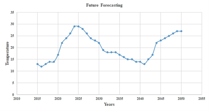
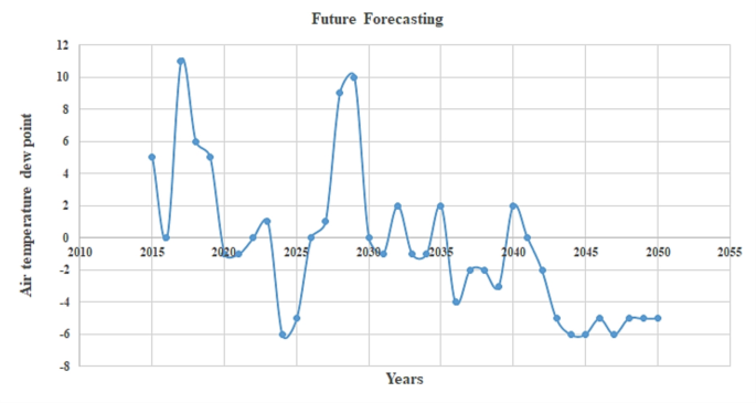
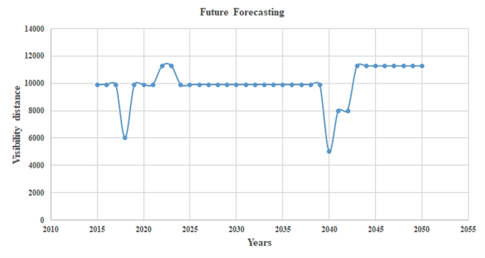
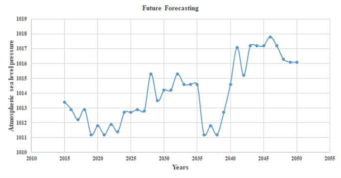
Figure 12 demonstrates the future forecasting for the temperature from 2015 to 2050 using the proposed CNN-GRU-LSTM model. From approximately 2015 to 2025, there is a rise in temperature, peaking at around 30. After 2025, the temperature drops significantly, reaching its lowest level around 2035. Between 2035 and 2040, the temperature remains stable with slight fluctuations. From 2040 to 2050, the temperature shows a rise in temperatures rising to around 25 by 2050. Figure 13 demonstrates the future forecasting for air temperature dew point from 2015 to 2050 using the proposed CNN-GRU-LSTM model. From 2015 to 2020, the dew point shows large fluctuations, with notable peaks in the period between 2015 and 2020, reaching values above 10. After 2020, the dew point trends downward, reaching a low near 2025, followed by a period of relative stability. Between 2025 and 2035, the dew point rises again, peaking near 12 around 2030, and then fluctuates. From 2035 to 2050, the dew point shows a gradual decrease with slight fluctuations, reaching a lowest level near − 7 around 2045, then stabilizing with slight changes towards 2050. Figure 14 demonstrates the future forecasting for visibility distance from 2015 to 2050 using the proposed CNN-GRU-LSTM model. The visibility distance remains constant around 10,000 in 2015. A sharp decline to approximately 6,000 is observed around 2015, followed by a return to stability. Between 2020 and 2025, oscillations appear in visibility, peaking slightly above 10,000 before stabilizing. From 2025 to 2035, the visibility distance consistently hovers around 10,000. Around 2040, another sharp decline occurred, with visibility dropping to around 4000. After this decline, visibility gradually recovers, stabilizing at around 12,000 from 2045 to 2050. Figure 15 demonstrates the future forecasting for atmospheric sea level pressure from 2015 to 2050 using the proposed CNN-GRU-LSTM model. Atmospheric sea level pressure starts at approximately 1013 in 2015, it shows a decreasing trend until approximately 2018. During the period from 2018 to 2025, the pressure shows large fluctuations characterized by many prominent peaks and troughs. After 2025, the pressure shows a marked upward trajectory that peaks around 2035. After 2035, the pressure continues to fluctuate periodically, with significantly higher peaks occurring around 2040 and 2045. When this period ends, the pressure stabilizes slightly above 1016.
