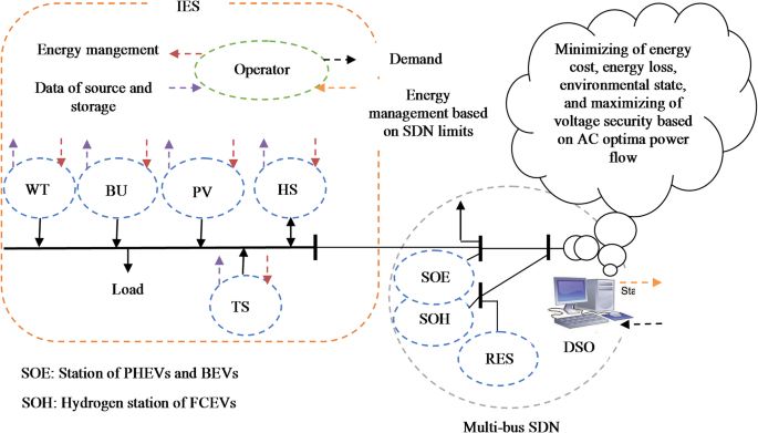
In this section, SDN energy management in the presence of renewable IES based on HS, BEV and PHEV charging stations, FCEV hydrogen station and renewable resources based on economic, operational, environmental and voltage security goals of DSO is expressed. The plan is presented as a multi-objective optimization problem, which its objective function is the minimizing the weighted sum of economic, operational, environmental and voltage security indicators. This plan is bound to the optimal power flow model and SDN security limitation, IES operation formulation and EV stations constraints. The details of this plan are explained below.
(A)
Objective function: Eq. (1) expresses the objective function of the proposed plan to minimize the weighted sum of expected energy cost (EEC)27, expected energy loss (EEL), expected pollution (EP)28 and voltage security index (VSI)27. EEC is modeled in relation (2). This relation refers to the total of SDN energy purchase cost from the upstream network, which at any moment is obtained by multyplying the energy price and the active power passing through the distribution post located in the slack bus connected to the upstream network (bus 1 is assumed here)26. EEL is formulated in relation (3). EEL is the difference between production and consumption energy in the operation horizon. EP has the same relationship as constraint (4). In this connection, EP equals the multiplication of the emission factor and the active power passing through the distribution substation connected to the upstream network. The emission coefficient is the sum of CO2, SO2 and NOx emission coefficients28. Equation (5) expresses the voltage security index, which is the ratio of the time sum of the WSI. The WSI is expressed for a weak bus in terms of voltage magnitude. A big WSI means that the conditions of voltage security in the SDN are optimal27.
$$\hbox{min} \,\,\,\,F={\xi _{EEC}}EEC+{\xi _{EEL}}EEL+{\xi _{EP}}EP+{\xi _{VSI}}VSI$$
(1)
where:
$$EEC=\sum\limits_{{h,s}} {\Delta T \times {\pi _s}{\lambda _{h,s}}P_{{n=1,h,s}}^{{DS}}}$$
(2)
$$\hbox{min} \,\,\,\,EEL=\sum\limits_{{n,h,s}} {\Delta T \times {\pi _s}\left( {P_{{n,h,s}}^{{DS}}+P_{{n,h,s}}^{{IES}}+P_{{n,h,s}}^{{RES}} – P_{{n,h,s}}^{{SOH}} – P_{{n,h,s}}^{{SOE}} – P_{{n,h,s}}^{C}} \right)}$$
(3)
$$EP=\sum\limits_{{h,s}} {\Delta T \times {\pi _s}{\gamma ^P}P_{{n=1,h,s}}^{{DS}}}$$
(4)
$$VSI= – \sum\limits_{{h,s}} {{\pi _s}WS{I_{h,s}}}$$
(5)
(B)
Formulation of SDN: SDN operating model bound to voltage security is expressed in relations (6)–(16). The constraints of network AC power flow are presented in relations (6)–(11), which indicates the active-reactive power balance in SDN buses29,30,31,32, active and reactive power passing through the distribution line, angle and magnitude of voltage in the slack bus (bus 1 is assumed here), respectively8,27. SDN operation limitations are modeled in constraints (12)–(15). In relation (12), the limit of the bus voltage magnitude is presented. Its lower (upper) limit is to prevent blackout of consumers (insulation damage of network equipment) due to high voltage drop (over-voltage)28. The functional limitation of the distribution post is stated in relation (13), so that the limitation of the distribution substation capacity is used in relation (13), and it refers to the limitation of the maximum apparent power passing through the distribution substation. In Eq. (14), the limit of the apparent power passing through the distribution lines is presented33,34,35,36. In this section, the SDN is assumed to have a distribution substation located at the slack bus. Hence, Eq. (13) is presented only for the slack bass. SDN voltage security constraints are expressed in relations (15) and (16)27. In this section, WSI is used to model voltage security. WSI is defined for the weakest bus in terms of voltage magnitude. This index has a value between 0 and 1. Zero represents voltage collapse, and unity represents SDN no-load condition27. The high level of WSI corresponds to the optimal conditions of voltage security in the distribution system. The WSI model is presented in Eq. (15), and its limit is formulated in (16).
$$P_{{n,h,s}}^{{DS}}+P_{{n,h,s}}^{{IES}}+P_{{n,h,s}}^{{RES}} – P_{{n,h,s}}^{{SOH}} – P_{{n,h,s}}^{{SOE}} – P_{{n,h,s}}^{C}=\sum\limits_{k} {C_{{n,k}}^{{EL}}P_{{n,k,h,s}}^{{EL}}\,\,\,\,\,} \,\,\,\,\forall n,h,s$$
(6)
$$Q_{{n,h,s}}^{{DS}} – Q_{{n,h,s}}^{C}=\sum\limits_{k} {C_{{n,k}}^{{EL}}Q_{{n,k,h,s}}^{{EL}}\,\,\,\,\,} \,\,\,\,\forall n,h,s$$
(7)
$$\begin{gathered} P_{{n,k,h,s}}^{{EL}}=G_{{n,k}}^{{EL}}{\left( {{V_{n,h,s}}} \right)^2} – {V_{n,h,s}}{V_{k,h,s}}\left( {G_{{n,k}}^{{EL}}\cos \left( {{\delta _{n,h,s}} – {\delta _{k,h,s}}} \right)+B_{{n,k}}^{{EL}}\sin \left( {{\delta _{n,h,s}} – {\delta _{k,h,s}}} \right)} \right) \hfill \\ \,\,\,\,\,\,\,\,\,\,\,\,\,\,\,\,\,\,\,\,\,\,\,\,\,\,\,\,\,\,\,\,\,\,\,\,\,\,\,\,\,\,\,\,\,\,\,\,\,\,\,\,\,\,\,\,\,\,\,\,\,\,\,\,\,\,\,\,\,\,\,\,\,\,\,\,\,\,\,\,\,\,\,\,\,\,\,\,\,\,\,\,\,\,\,\,\,\,\,\,\,\,\,\,\,\,\,\,\,\,\,\,\,\,\,\,\,\,\,\,\,\,\,\,\,\,\,\,\,\,\,\,\,\,\,\,\,\,\,\,\,\forall n,k,h,s \hfill \\ \end{gathered}$$
(8)
$$\begin{gathered} Q_{{n,k,h,s}}^{{EL}}= – B_{{n,k}}^{{EL}}{\left( {{V_{n,h,s}}} \right)^2}+{V_{n,h,s}}{V_{k,h,s}}\left( {B_{{n,k}}^{{EL}}\cos \left( {{\delta _{n,h,s}} – {\delta _{k,h,s}}} \right) – G_{{n,k}}^{{EL}}\sin \left( {{\delta _{n,h,s}} – {\delta _{k,h,s}}} \right)} \right) \hfill \\ \,\,\,\,\,\,\,\,\,\,\,\,\,\,\,\,\,\,\,\,\,\,\,\,\,\,\,\,\,\,\,\,\,\,\,\,\,\,\,\,\,\,\,\,\,\,\,\,\,\,\,\,\,\,\,\,\,\,\,\,\,\,\,\,\,\,\,\,\,\,\,\,\,\,\,\,\,\,\,\,\,\,\,\,\,\,\,\,\,\,\,\,\,\,\,\,\,\,\,\,\,\,\,\,\,\,\,\,\,\,\,\,\,\,\,\,\,\,\,\,\,\,\,\,\,\,\,\,\,\,\,\,\,\,\,\,\,\,\,\,\,\forall n,k,h,s \hfill \\ \end{gathered}$$
(9)
$${\delta _{n,h,s}}=0\,\,\,\,\,\,\,\,\,\,\forall n=1,h,s$$
(10)
$${V_{n,h,s}}=1\,\,\,\,\,\,\,\,\,\,\forall n=1,h,s$$
(11)
$$V_{n}^{{lo}} \leqslant {V_{n,h,s}} \leqslant V_{n}^{{up}}\,\,\,\,\,\,\,\,\,\,\forall n,h,s$$
(12)
$$\sqrt {{{\left( {P_{{n,h,s}}^{{DS}}} \right)}^2}+{{\left( {Q_{{n,h,s}}^{{DS}}} \right)}^2}} \leqslant \bar {S}_{n}^{{DS}}\,\,\,\,\forall n=1,h,s$$
(13)
$$\sqrt {{{\left( {P_{{n,k,h,s}}^{{EL}}} \right)}^2}+{{\left( {Q_{{n,k,h,s}}^{{EL}}} \right)}^2}} \leqslant \bar {S}_{{n,k}}^{{EL}}\,\,\,\,\forall n,k,h,s$$
(14)
$$\begin{gathered} WS{I_{h,w}}={\left( {{V_{n – 1,h,s}}} \right)^4} – 4{\left( {{V_{n – 1,h,s}}} \right)^2}\left( {{R_{n,n – 1}}P_{{n,n – 1,h,s}}^{{EL}}+{X_{n,n – 1}}Q_{{n,n – 1,h,s}}^{{EL}}} \right) \hfill \\ \,\,\,\,\,\,\,\,\,\,\,\,\,\,\, – 4{\left( {{X_{n,n – 1}}P_{{n,n – 1,h,s}}^{{EL}} – {R_{n,n – 1}}Q_{{n,n – 1,h,s}}^{{EL}}} \right)^2}\,\,\,\,\forall n=p,h,s \hfill \\ \end{gathered}$$
(15)
$$WS{I_{h,w}} \geqslant WS{I^{\hbox{min} }}\,\,\,\,\forall h,s$$
(16)
(C)
Operation of renewable IESs with HS: In relations (17)–(26), the performance model of renewable IESs based on hydrogen storage is presented. The balance of active power in IES corresponds to condition (17). Based on this relationship, the active power of IES from the view point of SDN (the active power of IES at the connection point to SDN) is equal to the sum of the active power produced by wind, solar, tidal, and bio-waste renewable sources, and H2P in HS minus the active power consumed by P2H in HS and passive loads. Equations (18)–(21) calculate the amount of production power obtained from renewable resources. In relation (18), the active power of the wind farm (WF) is modeled based on the wind speed3. The wind system has four working areas37,38,39,40,41. In the first (fourth) area, the wind speed is lower (higher) than the cut-in (cut-out) speed. In the second (third) area, the wind speed is between cut-in and nominal (nominal and cut-out) speed. In the first area, due to the low wind speed, power is not produced at the output of the wind system. In the second area, when wind speed rises, the active power generation increases linearly. In the third area, in order to prevent damage to the mechanical part of the wind system due to high wind speed, the production power of this system is kept constant at its capacity (the product of the number of wind turbines and the capacity of one turbine)3. Due to the high wind speed in the fourth area, a braking state is created and power is not produced at the output of the wind system. The production power model of the PV farm in terms of the sun irradiation is presented in Eq. (19)42. The active power produced in this farm is found by multiplying the number of PVs, the efficiency and surface of the PV panel, and the solar radiation on the surface of the PVs42,43,44,45,46,47. The production power of the BU farm in terms of gas obtained from bio-waste is modeled in relation (20)3. The production active power in the BU farm is found by multiplying the number of BUs, BU efficiency, percentage of methane in BU gas, low heat value for BU and BU gas production48. In relation (21), the performance model of TSs is presented49. It is noteworthy that TS has a wind turbine, the speed of the wind hitting to this turbine is the result of sea waves. Therefore, its functional model is the same as the wind farm in Eq. (10), with the difference that its wind speed is caused by sea waves49. Formulation of hydrogen storage operation is expressed in relations (22)–(26)4,8. A HS consists of P2H, H2P and a hydrogen tank (HT). P2H like an electrolyzer converts electrical energy into hydrogen. But H2P like a fuel cell converts hydrogen into electrical energy. The output hydrogen of P2H can be used to feed hydrogen loads such as hydrogen station of FCEVs, or it can be stored in HT8,50. H2P in HS receives hydrogen from HT and produces electrical energy in its output. The capacity limit of H2P and P2H is expressed in relations (22) and (23), respectively. In HS, P2H and H2P should not be active at the same time. This issue is modeled in constraint (24). Based on this condition, at any moment, the active power of H2P or P2H is equal to zero. It means that H2P or P2H is off at any moment. In relation (25), the amount of energy stored in HT is calculated. The energy stored in HT for each moment is equal to the sum of the energy stored in the previous time step, and the energy resulting from P2H activity minus the energy discharged by H2P and the hydrogen station of FCEVs8. In the first time-step, the energy stored in the previous time step is the initial energy of HT. Based on Eq. (25), it is assumed that IES by HS can feed part of the hydrogen of the FCEV station near the location of IES. In Eq. (26), the limit of energy stored in HT is modeled.
$$P_{{n,h,s}}^{{IES}}=P_{{n,h,s}}^{{WT}}+P_{{n,h,s}}^{{PV}}+P_{{n,h,s}}^{{BU}}+P_{{n,h,s}}^{{TS}}+\left( {P_{{n,h,s}}^{{H2P}} – P_{{n,h,s}}^{{P2H}}} \right) – P_{{n,h,s}}^{C}\,\,\,\,\forall n,h,s$$
(17)
$$P_{{n,h,s}}^{{WT}}=n_{n}^{{WT}}\bar {P}_{n}^{{WT}}\left\{ {\begin{array}{*{20}{c}} {0\,\,\,\,\,\,\,v_{n}^{{cin}} \geqslant v_{{n,h,s}}^{{WT}} \geqslant v_{n}^{{cout}}} \\ {\frac{{v_{{n,h,s}}^{{WT}} – v_{n}^{{cin}}}}{{v_{n}^{r} – v_{n}^{{cin}}}}\,\,\,\,\,\,\,v_{n}^{{cin}} \leqslant v_{{n,h,s}}^{{WT}} \leqslant v_{n}^{r}} \\ {1\,\,\,\,\,\,\,\,v_{n}^{r} \leqslant v_{{n,h,s}}^{{WT}} \leqslant v_{n}^{{cout}}} \end{array}} \right.\,\,\,\,\,\,\,\forall n,h,s$$
(18)
$$P_{{n,h,s}}^{{PV}}=n_{n}^{{PV}}\eta _{n}^{{PV}}A_{n}^{{PV}}I_{{n,h,s}}^{{PV}}\,\,\,\,\,\,\,\forall n,h,s$$
(19)
$$P_{{n,h,s}}^{{BU}}=n_{n}^{{BU}}\eta _{n}^{{BU}}\rho _{n}^{{BU}}LHV_{n}^{{BU}}G_{{n,h,s}}^{{BU}}\,\,\,\,\,\,\,\forall n,h,s$$
(20)
$$P_{{n,h,s}}^{{TS}}=n_{n}^{{TS}}\bar {P}_{n}^{{TS}}\left\{ {\begin{array}{*{20}{c}} {0\,\,\,\,\,\,\,v_{n}^{{cin}} \geqslant v_{{n,h,s}}^{{TS}} \geqslant v_{n}^{{cout}}} \\ {\frac{{v_{{n,h,s}}^{{TS}} – v_{n}^{{cin}}}}{{v_{n}^{r} – v_{n}^{{cin}}}}\,\,\,\,\,\,\,v_{n}^{{cin}} \leqslant v_{{n,h,s}}^{{TS}} \leqslant v_{n}^{r}} \\ {1\,\,\,\,\,\,\,\,v_{n}^{r} \leqslant v_{{n,h,s}}^{{TS}} \leqslant v_{n}^{{cout}}} \end{array}} \right.\,\,\,\,\,\,\,\forall n,h,s$$
(21)
$$0 \leqslant P_{{n,h,s}}^{{H2P}} \leqslant \bar {P}_{n}^{{H2P}}\,\,\,\,\forall n,h,s$$
(22)
$$0 \leqslant P_{{n,h,s}}^{{P2H}} \leqslant \bar {P}_{n}^{{P2H}}\,\,\,\,\forall n,h,s$$
(23)
$$P_{{n,h,s}}^{{H2P}}P_{{n,h,s}}^{{P2H}}=0\,\,\,\,\forall n,h,s$$
(24)
$$E_{{n,h,s}}^{{HT}}=\left\{ {\begin{array}{*{20}{c}} {\hat {E}_{n}^{{HT}}+\Delta T \times \left( {\eta _{n}^{{P2H}}P_{{n,h,s}}^{{P2H}} – \frac{1}{{\eta _{n}^{{H2P}}}}P_{{n,h,s}}^{{H2P}} – \eta _{n}^{{SOH}}P_{{n,h,s}}^{{SOH}}} \right)\,\,\,\,\,\,\,\,h=1} \\ {E_{{n,h – 1,s}}^{{HT}}+\Delta T \times \left( {\eta _{n}^{{P2H}}P_{{n,h,s}}^{{P2H}} – \frac{1}{{\eta _{n}^{{H2P}}}}P_{{n,h,s}}^{{H2P}} – \eta _{n}^{{SOH}}P_{{n,h,s}}^{{SOH}}} \right)\,\,\,\,h>1} \end{array}} \right.\,\,\,\,\,\,\,\,\forall n,s$$
(25)
$$\underset{\raise0.3em\hbox{$\smash{\scriptscriptstyle-}$}}{E} _{n}^{{HT}} \leqslant E_{{n,h,s}}^{{HT}} \leqslant \bar {E}_{n}^{{HT}}\,\,\,\,\,\,\,\,\forall n,h,s$$
(26)
(D)
Operation of EV stations: In this paper, it is assumed that a EV, when connected to a charging station, performs at charging mode with a constant charging rate equal to the charging station capacity. When its battery is full according to the EV owner’s request, the charging operation is interrupted. For example, a EV battery has a capacity of 40 kWh, and the charger capacity is 80 kW. If the a EV connects to charging station, the EV receives power of 80 kW from the charger and charges its battery in 30 min. This is true for fuel cell vehicles connected to a hydrogen station. Accordingly, in relations (27)–(29), the operation model of charging stations for BEVs and PHEVs is presented. Each station has several chargers, each charger can charge a BEV or PHEV in a certain period. Therefore, according to Eq. (27), the active power of the charging station is the sum of the active power of the chargers. It is assumed that each charger charges the mentioned EVs according to its capacity. Therefore, as in relation (28), the active power of the charger is zero or its capacity. In this equation, xCS is a binary parameter. Based on Eq. (29), this parameter has two values of zero and 1. The value of this parameter depends on the number of EVs (BEV or PHEV) connected to the charger. If a BEV or PHEV is connected to the charger, then xCS is equal to 1, but if no vehicle is connected to the charger, xCS is equal to zero. The operating model of the hydrogen station for FCEVs is expressed in relations (30)–(32). Its model is the same as BEV and PHEV charging station operation. Based on Eq. (30), the active power of each station is equal to the total active power of hydrogen pumps (include a P2H). The active power in each pump is equal to zero or its capacity based on Eq. (31). In other words, in this relation, xHS is a binary parameter that is calculated based on relation (32). The value of this parameter depends on the number of FCEVs in each hydrogen pump. So, if the pump feeds an FCEV, xHS is equal to 1, but if no FCEV is connected to the hydrogen pump, xHS has zero value. At hydrogen stations, FCEVs are generally fueled in 15 min. BEV has a large battery size, charging time is generally around 30 min. The PHEV has a smaller battery than the BEV, so its charging time is around 15 min. Hence, the time step (ΔT) in the proposed problem is equal to 15 min–0.25 h.
$$P_{{n,h,s}}^{{SOE}}=\sum\limits_{l} {P_{{n,l,h,s}}^{{CS}}\,\,\,\,\,} \,\,\,\,\forall n,h,s$$
(27)
$$P_{{n,l,h,s}}^{{CS}}=x_{{n,l,h,s}}^{{CS}}\bar {P}_{{n,l}}^{{CS}}\,\,\,\,\forall n,l,h,s$$
(28)
$$x_{{n,l,h,s}}^{{CS}}=\left\{ {\begin{array}{*{20}{c}} {1\,\,\,\,\,\,N_{{n,l,h,s}}^{{EV}} \ne 0} \\ {0\,\,\,\,\,\,N_{{n,l,h,s}}^{{EV}}=0} \end{array}} \right.\,\,\,\,\,\,\,\forall n,l,h,s$$
(29)
$$P_{{n,h,s}}^{{SOH}}=\sum\limits_{t} {P_{{n,t,h,s}}^{{HS}}\,\,\,\,\,} \,\,\,\,\forall n,h,s$$
(30)
$$P_{{n,t,h,s}}^{{HS}}=x_{{n,t,h,s}}^{{HS}}\bar {P}_{{n,t}}^{{HS}}\,\,\,\,\forall n,t,h,s$$
(31)
$$x_{{n,t,h,s}}^{{HS}}=\left\{ {\begin{array}{*{20}{c}} {1\,\,\,\,\,\,N_{{n,t,h,s}}^{{FCEV}} \ne 0} \\ {0\,\,\,\,\,\,N_{{n,t,h,s}}^{{FCEV}}=0} \end{array}} \right.\,\,\,\,\,\,\,\forall n,t,h,s$$
(32)
(E)
Determining the compromise solution: In relation (1), the parameters ξEEC, ξEEL, ξEP and ξVSI respectively represent the weight coefficient of EEC, EEL, EP and VSI in the objective function (1). Each of the coefficients can vary in the range of 0 and 1, and their sum must also be 1. When the coefficients have different values, then different quantities are obtained for EEC, EEL, EP and VSI functions. Drawing these functions in 4-dimensional coordinates shows the Pareto front of the plan. This front indicates that there are many optimal points for the proposed design. In the upcoming paragraphs, the fuzzy decision-making method extracts an optimal point that corresponds to the compromise point between different functions28. In this method, first the proposed problem is solved for four cases ξEEC = 1, ξEEL = 1, ξEP = 1 and ξVSI = 1, which are respectively the minimum value (Fmin) of EEC, EEL, EP and VSI functions, respectively. In these four cases, the maximum value (Fmax) of the mentioned functions is also calculated. Then, for different values of weight coefficients, the amount of fuzzy linear membership function (\(\overset{\lower0.5em\hbox{$\smash{\scriptscriptstyle\frown}$}}{f}\)) for the mentioned functions is calculated based on Eq. (33)28. Based on this relationship, if a function (F) has a value less (more) than Fmin (Fmax), the value of \(\overset{\lower0.5em\hbox{$\smash{\scriptscriptstyle\frown}$}}{f}\)is 1 (0). Otherwise, it is (F – Fmax)/(Fmin – Fmax). In relation (33), nPF represents the number of members of the Pareto front. i represents the member of the Pareto front, j represents the index of different functions in the objective function. Next, the minimum value of \(\overset{\lower0.5em\hbox{$\smash{\scriptscriptstyle\frown}$}}{f}\) between different functions is determined based on Eq. (34), which is considered equal to ϕ. Finally, based on relation (35), the compromise point (CP) corresponds to the point with the largest ϕ28. The flowchart of the fuzzy decision-making method for the proposed design is presented in Fig. 2.
$${\overset{\lower0.5em\hbox{$\smash{\scriptscriptstyle\frown}$}}{f} _{i,j}}=\left\{ {\begin{array}{*{20}{c}} {1\,\,\,\,\,\,\,\,\,\,\,\,\,\,\,\,\,\,\,\,\,\,\,\,\,\,\,F_{{i,j}}^{{\hbox{min} }} \geqslant {F_{i,j}}} \\ {\frac{{{F_{i,j}} – F_{{i,j}}^{{\hbox{max} }}}}{{F_{{i,j}}^{{\hbox{min} }} – F_{{i,j}}^{{\hbox{max} }}}}\,\,\,\,\,F_{{i,j}}^{{\hbox{min} }} \leqslant {F_{i,j}} \leqslant F_{{i,j}}^{{\hbox{max} }}} \\ {0\,\,\,\,\,\,\,\,\,\,\,\,\,\,\,\,\,\,\,\,\,\,\,\,{F_{i,j}} \geqslant F_{{i,j}}^{{\hbox{max} }}} \end{array}\,\,\,\,\,\,\,\,\forall i \in \{ 1,2,.,{n_{PF}}\} ,j \in \{ EEC,EEL,EP,VSI\} } \right.$$
(33)
$${\varphi _i}=\hbox{min} \left( {{{\overset{\lower0.5em\hbox{$\smash{\scriptscriptstyle\frown}$}}{f} }_{i,j=EEC}},{{\overset{\lower0.5em\hbox{$\smash{\scriptscriptstyle\frown}$}}{f} }_{i,j=EEL}},{{\overset{\lower0.5em\hbox{$\smash{\scriptscriptstyle\frown}$}}{f} }_{i,j=EP}},{{\overset{\lower0.5em\hbox{$\smash{\scriptscriptstyle\frown}$}}{f} }_{i,j=VSI}}} \right)\,\,\,\,\forall i$$
(34)
$$CP=\hbox{max} \left( {{\varphi _1},{\varphi _2},.,{\varphi _{{n_{PF}}}}} \right)$$
(35)

Flowchart of the fuzzy decision-making method for the proposed plan.