Concatenate codes, save qubits | npj Quantum Information

In Methods, after summarizing the notations, we first describe the error model used in the numerical simulation and the Monte Carlo simulation method to evaluate the logical CNOT error rate. Then, we provide the details of our estimation of the required logical error rate of quantum computation, based on the evaluation of the CNOT gate counts of the quantum circuit implementing Shor’s algorithm for 2048-bit RSA integer factoring and the required error rates for the classical computation. Finally, we present our method for estimating the logical CNOT error rate of the large-scale concatenated codes using the small-scale level-by-level simulation results at each concatenation level.

Notation

The computational basis (also called the Z basis) of a qubit \({{\mathbb{C}}}^{2}\) is denoted by \(\{\left\vert 0\right\rangle ,\left\vert 1\right\rangle \}\), and the complementary basis (also called the X basis) \(\{\left\vert +\right\rangle ,\left\vert -\right\rangle \}\) is defined by \(\left\vert \pm \right\rangle :=\frac{1}{\sqrt{2}}(\left\vert 0\right\rangle \pm \left\vert 1\right\rangle )\). By the convention of ref. 52, we use the following notation on 1-qubit and 2-qubit unitaries:

where the 1-qubit and 2-qubit unitaries are shown in the matrix representations in the computational bases \(\{\left\vert 0\right\rangle ,\left\vert 1\right\rangle \}\subset {{\mathbb{C}}}^{2}\) and \(\{\left\vert 0\right\rangle \otimes \left\vert 0\right\rangle ,\left\vert 0\right\rangle \otimes \left\vert 1\right\rangle ,\left\vert 1\right\rangle \otimes \left\vert 0\right\rangle ,\left\vert 1\right\rangle \otimes \left\vert 1\right\rangle \}\subset {{\mathbb{C}}}^{2}\otimes {{\mathbb{C}}}^{2}\), respectively. See also ref. 53 for terminology on FTQC.

Error model

In this work, the stabilizer circuits for describing the fault-tolerant protocols are composed of state preparations of \(\left\vert 0\right\rangle\) and \(\left\vert +\right\rangle\), measurements in the Z and X bases, single-qubit gates I, X, Y, Z, H, S, and a two-qubit CNOT gate. Each of these preparation, measurement, and gate operations in a circuit is called a location in the circuit. By the convention of ref. 12, we use a circuit-level depolarizing error model. In this model, independent and ideally distributed (IID) Pauli errors randomly occur at each location, i.e., after state preparations and gates, and before measurements. By convention, we ignore the error and the runtime of polynomial-time classical computation used for decoding in the fault-tolerant protocols.

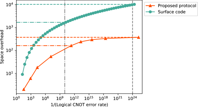
The probabilities of the errors are given using a single parameter p (called the physical error rate) as follows. State preparations of \(\left\vert 0\right\rangle\) and \(\left\vert +\right\rangle\) are followed by X and Z gates, respectively, with probability p. Measurements in Z and X bases follow X and Z gates, respectively, with probability p. One-qubit gates I, X, Y, Z, H, S are followed by one of the 3 possible non-identity Pauli operators {X, Y, Z}, each with probability p/3. A two-qubit gate CNOT is followed by one of the 15 possible non-identity Pauli products acting on 2 qubits \({\{{\sigma }_{1}\otimes {\sigma }_{2}\}}_{({\sigma }_{1},{\sigma }_{2})\in {\{I,X,Y,Z\}}^{2}}\setminus \{I\otimes I\}\), each with probability p/15. We also investigate different error models, where the Pauli error rate on the identity gate I is changed from p/3 to γ/3, where γ is taken to be γ = p/2 and γ = p/10. As shown in Fig. 4, our protocol, shown in Table 1 significantly reduces the space overhead compared to that for the surface code in these error models (see Supplementary Information for more details).

Fig. 4: Comparison of space overhead of the proposed protocol with that for the surface code under three error models (γ = p, γ = p/2 and γ = p/10).

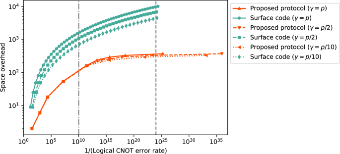
The figure plots the space overheads and logical error rates of the proposed protocol shown in Table 1 (▴ for γ = p, ▾ for γ = p/2 and ◂ for γ = p/10) and the surface code (• for γ = p, ■ for γ = p/2 and ♦ for γ = p/10). The plots for the error model γ = p are the same as shown in Fig. 1. The logical error rate is calculated under a circuit-level depolarizing error model at a physical error rate 0.1%. The dash-dotted and lines represent the logical error rate 10−10 and 10−24, respectively. Our protocol reduces the space overhead compared to the protocol for the surface code in a similar magnitude as in the error model used in Fig. 1.

Simulation to evaluate logical CNOT error rates

In our numerical simulation, we evaluate the logical CNOT error rate using the Monte Carlo sampling method presented in refs. 21,22, which is based on the reference entanglement method13,23. For a quantum code consisting of N physical qubits and K logical qubits, the circuit that we use for the Monte Carlo sampling method is illustrated in Fig. 5, where we assume that random Pauli errors occur at each location of the circuit according to the error model described above. In particular, starting from two error-free logical Bell states, we repeatedly apply a gate gadget of the logical CNOT⊗K gate, followed by an error correction gadget, which is repeated ten times. For all the quantum codes (which are Calderbank-Shor-Steane (CSS) codes in this work) except for the surface code, we implement the logical CNOT gates transversally and use Knill’s error correction gadget13 for error correction. Note that Steane’s error correction gadget53,54 may also have a similar performance to Knill’s, but in practice, Knill’s error correction gadget is more robust to leakage errors than Steane’s55 and thus is preferable to use if possible. We also note that the addressable CNOT gate can be performed via gate teleportation using a certain stabilizer state56, and the threshold of the distillation of a logical stabilizer state is much larger than that of the logical CNOT gate. Therefore, we expect the threshold of the addressable CNOT gate is comparable with that of the transversal CNOT gate. For the surface code, by convention, we use the lattice surgery31,32 to implement the logical CNOT gates, which includes the error correction. Note that the transversal implementation of the logical CNOT gate is also possible for the surface code57, but we performed our numerical simulation based on the lattice surgery since the lattice surgery is more widely used in the literature on resource estimation for FTQC, such as refs. 58,59, and the threshold of the lattice surgery CNOT is better than the transversal CNOT, as shown in ref. 57. Then, we apply the error-free logical Bell measurement on the output quantum state. Any measurement outcomes that do not result in all zeros for the kth logical qubits in four code blocks are counted as logical errors on the kth logical qubit for k ∈ {1, …, K}. We evaluate the logical CNOT error rate by dividing the empirical logical error probability in the simulation by ten and averaging over the K logical qubits. Since the quantum circuit in Fig. 5, including Pauli errors, is composed of Clifford gates, the sampling of measurement outcomes is efficiently simulated by a stabilizer circuit simulator; in particular, our simulation is conducted with STIM60.

Fig. 5: A quantum circuit for the reference entanglement method13,21,22,23 to estimate a logical CNOT error rate.

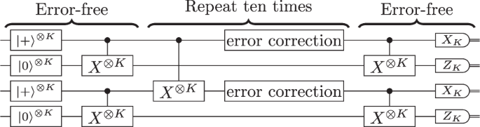
In this simulation, starting from two error-free logical Bell states, we apply a gate gadget of the logical CNOT⊗K gate, followed by the error correction gadget ten times, using a noisy circuit. For the surface code, we use the lattice surgery31,32 to implement logical CNOT gates, which includes the error correction. For the other codes, we implement logical CNOT gates transversally and use Knill’s error correction gadget13 for error correction. Finally, we apply the error-free logical Bell measurement on the output quantum state to estimate the logical error rate. The symbol with XK (ZK) denotes the measurements in X (Z) basis for all the K logical qubits in a code block.

Logical error rate required for 2048-bit RSA integer factoring

The security of the RSA cryptosystem is ensured by the classical hardness of integer factoring, and factoring 2048-bit integers given as the product of two similar-sized prime numbers, which is called RSA integers in ref. 25 leads to breaking RSA-2048. Previous works have investigated efficient algorithms for RSA integer factoring based on Shor’s algorithm24. In particular, ref. 25 proposes an n-bit RSA integer factoring algorithm using 0.3n3 + 0.0005n3lg n Toffoli gates. Since a Toffoli gate can be decomposed into 6 CNOT gates and single-qubit gates52, this algorithm can be implemented by 1.8n3 + 0.003n3lg n CNOT gates. For n = 2048, it requires ~1010 CNOT gates. Thus, we require a logical error rate ~10−10 to run this algorithm.

Required error rate for classical computation

The required error rate for classical computation is estimated by taking an inverse of the number of elementary gates in a large-scale classical computation that is currently available. In particular, we consider a situation where the supercomputer Fugaku61 is run for a month. The peak performance at double precision of Fugaku in the normal mode is given as 488 petaflops ~5 × 1017 s−1 61. If we run it for 1 month ~2.6 × 106 s, then the number of elementary gates is roughly estimated as ~1024. Thus, an upper bound of the logical error rate of classical computation is roughly estimated as ~10−24.

Estimation of logical error rates of large-scale quantum codes from small-scale level-by-level simulations

In this work, we use an underlying quantum code \({{\mathcal{Q}}}_{0}\) concatenated with a series of quantum Hamming codes \({{\mathcal{Q}}}_{{r}_{1}},{{\mathcal{Q}}}_{{r}_{2}},\ldots ,{{\mathcal{Q}}}_{{r}_{L}}\). The logical error rate of the overall quantum code under the physical error rate p is evaluated from the level-by-level numerical simulation as

where P0(p) is the logical error rate of \({{\mathcal{Q}}}_{0}\) under the physical error rate p, and \({P}_{{r}_{l}}^{({r}_{l+1})}(p)\) is that of the quantum Hamming code \({{\mathcal{Q}}}_{{r}_{l}}\). Note that the protocol depends on the quantum code concatenated above (i.e., \({{\mathcal{Q}}}_{{r}_{l+1}}\)), thus the logical error rate of the level-l protocol depends on rl and rl+1 (see ref. 4 for the details). For the top code \({{\mathcal{Q}}}_{{r}_{L}}\), we implement the protocol such that we can concatenate the quantum code \({{\mathcal{Q}}}_{{r}_{L}+1}\) if needed. Thus, the logical error rate on the top code \({{\mathcal{Q}}}_{{r}_{L}}\) is evaluated as \({P}_{{r}_{L}}^{({r}_{L}+1)}\). This estimation gives the upper bound of the logical error rate in the cases where the logical CNOT gates (rather than initial-state preparation of \(\left\vert 0\right\rangle\) and \(\left\vert +\right\rangle\), single-qubit Pauli and Clifford gates, and measurements in Z and X bases) have the largest error rate in the set of elementary operations for the stabilizer circuits, which usually holds true since the gadget for the CNOT gate is the largest. The logical error rates P0(p) and \({P}_{{r}_{l}}(p)\) for each l ∈ {1, …, L} are estimated by the numerical simulation using the circuit described in Fig. 5. See Supplementary Information for more details.

With our numerical simulation, we obtain the parameters of the following fitting curves of the logical error rates (see Supplementary Information for more details). For the quantum Hamming code \({{\mathcal{Q}}}_{{r}_{l}}\) with parameter rl, due to distance 3, Pr(p) is approximated for \({r}_{l}\in \{3,4,5,6,7\},{r}_{l+1}\in \{{r}_{l}+1,\ldots ,\max ({r}_{l}+1,7)\}\) by the following fitting curve

The logical error rate of the level-l C4/C6 code, denoted by \({P}_{{C}_{4}/{C}_{6}}^{(l)}(p)\), is approximated by a fitting curve

where Fl is the Fibonacci number defined by F1 = 1, F2 = 2, and Fl = Fl−1 + Fl−2 for l > 213. The threshold \({p}_{{C}_{4}/{C}_{6}}^{({\rm{th}})}\) for the C4/C6 code is estimated by

The logical error rate of the surface code with code distance d, denoted by \({P}_{{\rm{surface}}}^{(d)}(p)\), is approximated by a fitting curve

Based on the critical exponent method in ref. 62, the threshold \({p}_{{\rm{surface}}}^{({\rm{th}})}\) of the surface code is estimated as a fitting parameter of another fitting curve given by

The logical error rate of the level-l concatenated Steane code, denoted by \({P}_{{\rm{Steane}}}^{(l)}(p)\), is approximated for l ∈ {1, 2} by a fitting curve

For l ≥ 3, due to the limitation of computational resources, we did not directly perform the numerical simulation to determine \({a}_{{\rm{Steane}}}^{(l)}\) in (17), but using the results for l ∈ {1, 2} in (17), we recursively evaluate the logical error rates \({P}_{{\rm{Steane}}}^{(l)}(p)\) of level-l concatenated Steane code as

The threshold \({p}_{{\rm{Steane}}}^{({\rm{th}})}\) of the concatenated Steane code is estimated by that satisfying \({P}_{{\rm{Steane}}}^{(2)}({p}_{{\rm{Steane}}}^{({\rm{th}})})={p}_{{\rm{Steane}}}^{({\rm{th}})}\), i.e.,

The logical error rates of the level-l C4/Steane codes for l ∈ {1, 2}, denoted by \({P}_{{C}_{4}/{\rm{Steane}}}^{(l)}(p)\), are approximated by fitting curves

where \({a}_{{C}_{4}/{\rm{Steane}}}^{(1)}\) is given by \({a}_{{C}_{4}/{\rm{Steane}}}^{(1)}={A}_{{C}_{4}/{C}_{6}}{B}_{{C}_{4}/{C}_{6}}\) from the logical error rate of the level-1 C4/C6 since the level-1 C4/Steane code coincides with the level-1 C4/C6 code. For l ≥ 3, similar to the concatenated Steane code, logical error rates \({P}_{{C}_{4}/{\rm{Steane}}}^{(l)}(p)\) of the level-l C4/Steane code are evaluated by

Since the C4/Steane code at concatenation levels 2 and higher becomes the same as the concatenated Steane code, the threshold \({p}_{{C}_{4}/{\rm{Steane}}}^{({\rm{th}})}\) of the C4/Steane code is determined by the physical error rate that can be suppressed below \({p}_{{\rm{Steane}}}^{({\rm{th}})}\) at level 2, estimated as that satisfying \({P}_{{C}_{4}/{\rm{Steane}}}^{(2)}({p}_{{C}_{4}/{\rm{Steane}}}^{({\rm{th}})})={p}_{{\rm{Steane}}}^{({\rm{th}})}\), i.e.,

Using the fitting parameters of these fitting curves obtained from the level-by-level numerical simulations, we evaluate the overall logical error rate according to (10).