This section describes the study area, data sources, and gathered data, followed by a brief mathematical explanation of the algorithms of interest is provided. Also, the metrics used to evaluate the experiments are presented.
Study area and data
Mar Menor is a coastal lagoon located in the Region of Murcia, Spain, with a surface area of 170 km2, a coastline length of 73 km, and a maximum depth of 7 m. The lagoon is separated from the Mediterranean Sea by a narrow strip of land known as La Manga.
The lagoon is characterized by its shallow waters, which are typically warmer than the adjacent Mediterranean Sea. The climate is semi-arid and characterized by hot, dry summers where daytime temperatures range from 30 to 40 degrees Celsius. Winters are mild, with temperatures between 10 and 20 degrees Celsius, and frost or snow is rare.
In this study, the source data are extracted from the Automatic Hydrological Information System (SAIH) of the Segura River Hydrographic Basin. It provides information on the levels and flows of the major rivers and tributaries, the levels and volumes impounded in the dams, the flows released through spillways, valves and gates, the precipitation at numerous points, and the flows withdrawn by the major water uses in the basin. As shown in Fig. 1, two main types of locations are used for this study. The stream gauge areas (stations starting with the code 06A*), in which the variables streamflow \(\hbox {(m}^{3}\hbox {/s)}\) and rain gauges (mm) are selected to develop this work, and the piezometers (also referred to as Sondeos and start with the code 06Z*), in which the piezometric level (msnm) is used. All variables used in this study are publicly available at https://www.chsegura.es/es/cuenca/redes-de-control/saih/ivisor/ (Accessed December 4, 2023) and are measured every five minutes. Measurements are obtained from the Confederación Hidrográfica del Segura (CHS), the official Spanish authority responsible for managing water resources in the Segura River basin. CHS ensures high-quality measurement standards and the maintenance of sensors and devices throughout the basin. A Python script is implemented to download the required data from the web page and then save it in Parquet format for more efficient data storage.
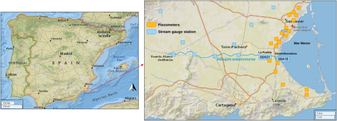
Map of all the sites used in this study in the Region of Murcia. The yellow points indicate the piezometers and the blue points the stream gauge stations. The blue line represents the Albujón watercourse. Map generated by the authors using Folium36, an interactive mapping library for Python based on Leaflet.js. The specific map layer used is Esri.NatGeoWorldMap from Leaflet Providers37.
Regarding the distribution of stream gauge station, location 06A18 (Desembocadura Rambla de Albujón) is the primary contributor to the Mar Menor, followed by location 06A01 (La Puebla) due to their proximity to the basin. For this work, data from a total of 12 stream gauge stations was used, with the importance of the stream gauge decreasing as one moves away from the main entrance to the Mar Menor. On the other hand, the piezometers are located to the west of the Mar Menor coast, with a total of 19 points. The stream gauge data cover a spatial area of 423.12 km2, with records starting from January 8, 2016, while the piezometer data cover 41.06 km2, with records starting from December 13, 2019. To develop reliable predictive models, data from March 8, 2021 (12:00 PM) to November 18, 2023 (11:55 PM) was isolated, ensuring a sufficient availability of streamflow records at the two focal points.
Methods
In this subsection, the ML and DL models employed in our study are outlined, including their respective definitions and parameter configurations.
Decision trees (DT) and random forest (RF)
A Decision Tree is a tree-like model used for both classification and regression. It partitions the data into subsets based on the features’ values, creating a tree structure where each node represents a feature, and each branch represents a decision rule. For a given observation \(x_i\) with m features each decision node \(j\) in a tree applies a split on a feature \(f_j\) using a threshold \(t_j\) as follows: \(\text {if } x_i[f_j] \le t_j \text { then } \text {left branch, else right branch}\). Terminal nodes (leaves) contain the predicted value.
Random Forest was first introduced by38 and is an ensemble learning method that constructs a multitude of DTs during training. It outputs the average prediction of individual trees for regression tasks or uses voting for classification. Each tree in the forest is trained on a random subset of the dataset, introducing randomness to enhance performance and reduce overfitting.
For regression tasks, the predicted output \(\hat{Y}\) for a new observation \(x\) is calculated as the average of predictions from individual trees. For classification tasks, it operates through a process of majority voting among the trees.
K-nearest neighbors (KNN)
KNeighbors is one of the fundamental algorithms in ML. KNN is an instance-based learning algorithm used for both classification and regression tasks. KNN utilizes the entire training dataset for both classification and regression tasks. When a new data point needs to be classified or assigned a value, KNN identifies the k closest neighbors to this point from the training dataset39. In classification tasks, it calculates the distance between the new point and the existing ones using metrics like Euclidean, Manhattan, or other distance measures and once the k nearest neighbours are identified, the most frequently occurring class label among them is assigned to the new point. In regression tasks, the process is similar, but instead of assigning a class label, KNN assigns the new point the average value of its k nearest neighbors. KNN has been previously applied in marine science-related problems40.
Linear regression (LR) and Ridge regression (L2)
Linear Regression is a fundamental statistical technique that models the relationship between a dependent variable and one or more independent variables by fitting a linear equation to observed data.
Ridge Regression, also known as L2 regression, is a regularized linear regression technique that adds a penalty term proportional to the square of the magnitude of coefficients, thus helps control overfitting by shrinking the coefficients toward zero41. The formula is as follows:
\(\text {Minimize } \sum _{i=1}^{n} \left( y_i – (\beta _0 + \beta _1x_{i1} + \beta _2x_{i2} + \cdots + \beta _px_{ip}) \right) ^2 + \lambda \sum _{j=1}^{p} \beta _j^2\), where
\(y_i\): Represents the observed value of the dependent variable for the \(i^{th}\) observation.
\(x_{i1}, x_{i2}, \ldots , x_{ip}\): Represent the values of independent variables for the \(i^{th}\) observation.
\(\beta _0, \beta _1, \ldots , \beta _p\): Are the coefficients to be estimated.
p: Denotes the number of independent variables.
\(\lambda\): Is the regularization parameter controlling the penalty term. An increase in \(\lambda\) leads to stronger regularization and greater shrinkage of coefficients.
Gradient boosting (GB) and extreme gradient boosting (XGB)
Gradient Boosting is an ensemble technique that builds a model in a stage-wise manner by combining weak learners, typically decision trees, to improve predictive accuracy. It minimizes errors by iteratively fitting new models to the residual errors of previous models.
Extreme Gradient Boosting is an optimized and efficient implementation of Gradient Boosting designed for speed and performance42. It employs a more regularized model formalization to control overfitting and provides various hyperparameters for fine-tuning.
Neural networks for time series: long-short term neural network (LSTM)
LSTMs are a type of recurrent neural network (RNN) architecture designed to handle the vanishing and exploding gradient problems that are present in more traditional RNNs. The original paper presenting the standard LSTM cell concept was published in 199743. LSTMs excel at capturing long-range dependencies in sequential data, making them well-suited for time series analysis, natural language processing, and other sequential tasks. LSTMs contain memory cells that maintain information over extended time intervals, selectively remembering or forgetting information through specialized gates. They consist of input, forget, and output gates, enabling the model to regulate the flow of information within the network.
The forget gate, introduced by44, determines which information is retained or discarded from the cell state. When the forget gate value, \(f_t\), is 1, the information is retained; when it is 0, the information is discarded. Figure 2, illustrates the structure of an LSTM with a forget gate. The LSTM cell can be mathematically expressed as follows:
$$\begin{aligned} f_t&= \sigma (W_f \cdot h_{t-1} + W_f \cdot x_t + b_f), \end{aligned}$$
(1)
$$\begin{aligned} i_t&= \sigma (W_{ih} \cdot h_{t-1} + W_{ix} \cdot x_t + b_i), \end{aligned}$$
(2)
$$\begin{aligned} \tilde{c}_t&= \tanh (W_{\tilde{c}h} \cdot h_{t-1} + W_{\tilde{c}x} \cdot x_t + b_{\tilde{c}}), \end{aligned}$$
(3)
$$\begin{aligned} c_t&= f_t \cdot c_{t-1} + i_t \cdot \tilde{c}_t, \end{aligned}$$
(4)
$$\begin{aligned} o_t&= \sigma (W_{oh} \cdot h_{t-1} + W_{ox} \cdot x_t + b_o), \end{aligned}$$
(5)
$$\begin{aligned} h_t&= o_t \cdot \tanh (c_t). \end{aligned}$$
(6)
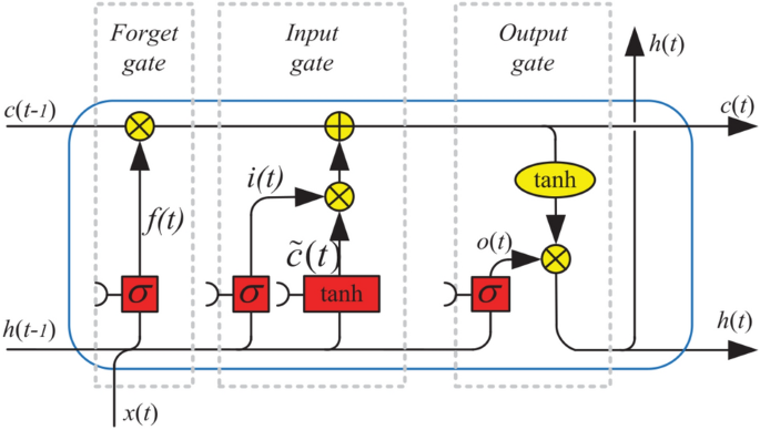
Architecture of LSTM with a forget gate. Image extracted from45.
Throughout our experiments, these ML models were implemented and automatically tuned with appropriate hyperparameters to address our research objectives and optimize predictive performance.
The selection of algorithms was based on their ability to handle the complexities of the data. Specifically, RF is robust in capturing nonlinear relationships and has demonstrated success in short-term streamflow prediction studies46. LSTM networks were chosen due to their architecture’s capability to process sequential data, making them ideal for capturing temporal dependencies in streamflow time series24. Finally, other algorithms, such as Gradient Boosting, K-Nearest Neighbors, and Linear Regression, were included to serve as comparative benchmarks, highlighting the advantages of ensemble and sequential models.
Metrics
This work assesses model accuracy using the following error metrics: the Nash–Sutcliffe Model Efficiency Coefficient (NSE)47, the reformulation of Willmott’s Index of agreement48, Root-Mean-Square Error (RMSE), Coefficient of the Variation of the Root Mean Square Error (CVRMSE) and Mean Absolute Error (MAE).
NSE is usually defined as:
$$\begin{aligned} \text {NSE} = 1 – \frac{\sum _{i=1}^{n}(Q_{o}- Q_{p})^2}{\sum _{i=1}^{n}(Q_{o}- \bar{Q}_{o})^2} \end{aligned}$$
(7)
where \(\bar{Q}_{o}\) is the mean value of observed streamflow, \(Q_p\) is the predicted streamflow and \(Q_{o}\) is the real streamflow. A perfect model would have an NSE of 1. An NSE of 0 means the model has the same predictive capacity as the mean of the time series, while a negative NSE indicates that the mean is a better predictor than the model.
The Willmott’s Index (WI) is calculated as follows:
$$\begin{aligned} \text {WI} = 1 – \frac{\sum _{i=1}^{n} (Q_{o} – Q_{p})^2}{\sum _{i=1}^{n} (| Q_{p} – \bar{Q}_{o}| + |Q_{o} – \bar{Q}_{o}|)^2} \end{aligned}$$
(8)
This index can take values between 0 and 1 and it represents the ratio of the mean square error and the potential error. Since NSE and WI consider square differences both metrics are overly sensitive to extreme values.
The RMSE is computed using the predictions \(Q_{p}\) and the real values \(Q_{o}\):
$$\begin{aligned} \text {RMSE} = \sqrt{\frac{1}{n}\sum _{t=1}^{n}\left( Q_{p} – Q_{o}\right) ^2} \end{aligned}$$
(9)
It has the same units as the predicted variable, allowing an intuitive understanding of prediction error magnitude.
CVRMSE can be computed with the RMSE:
$$\begin{aligned} \text {CVRMSE} = \frac{RMSE}{\bar{{Q}_{o}}}\times 100 \end{aligned}$$
(10)
CVRMSE is a dimensionless measure, where values close to 0 indicate better model performance. For example, a CVRMSE of 5% means that the mean unexplained variation in the real magnitude is 5% of its mean value49.
Finally, calculate the MAE as:
$$\begin{aligned} \text {MAE} = \frac{1}{n}\sum _{i=1}^{n}|Q_{p}-Q_{o}| \end{aligned}$$
(11)
Like RMSE, MAE has the same scale as the evaluated values, but it should not be used to compare predictions across different scales.