Ozone formation is more active on days with higher temperatures and stronger sunlight34, and ozone concentrations are generally higher during warm seasons (April to September) compared to cold seasons. Thus, our study focused on the warm seasons, consistent with previous research on ozone exposure and health impacts16,35,36.
We collected all OHCA cases from the Out-of-Hospital Cardiac Arrest Surveillance database for the warm seasons from 2015 to 2019, provided by the Korea Disease Control and Prevention Agency. This database includes information on OHCA onset dates, outcomes, age, sex, medical history, and OHCA onset locations. Our study population consisted of all OHCA cases occurring between April 1, 2015, and September 30, 2019. All variables of the OHCA surveillance including medical history status were based on medical records written by medical doctors. Moreover, the criteria for OHCA were “patients whose main symptoms are recorded by 119 emergency medical records”. Specifically, the OHCA cases were defined as 1) “cardiac arrest” or “respiratory arrest” in the emergency activity log, who have performed “cardiopulmonary resuscitation” for emergency treatment, or who has written a “Detailed Status Table for First Aid for Cardiopulmonary Suspension Patients” by emergency service operators.
Study design
We employed a time-stratified case-crossover design. The date of OHCA incidence served as the case date. For each case, we identified control days by matching the same day of the week, month, and year. This self-matching controlled for confounding variables that remain relatively stable within a month, such as age, sex, body mass index, health behaviors (e.g., diet and exercise), and regional factors (urbanicity, medical service accessibility, climate, and socioeconomic environment). Matching by day of the week addressed potential within-week differences, and bidirectional matching minimized biases from long-term exposure trends37. Matching by the same month within the same year controlled for seasonality and long-term trends. This standardized approach has been widely used to assess short-term environmental exposure risks to health outcomes38,39.
Air pollution and environmental data
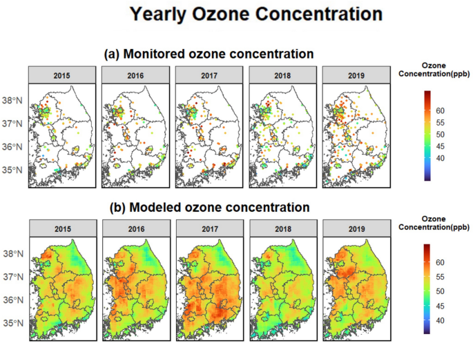
We used a nationwide modeled air pollution dataset, which includes high-resolution (1 km2) ozone (maximum 8-h average [ppb]) and PM2.5 (24-h average [µg/m3]) predictions from 2015 to 2019. The AiMS-CREATE team provided the modeled daily ozone concentrations across inland South Korea30. These predictions were generated using a machine-learning ensemble model incorporating random forest, extreme gradient boosting, and deep neural network algorithms based on satellite-based variables. Detailed information about the ensemble prediction model is available in the Supplemental Materials, “1. Air Pollution Prediction Models.” The models demonstrated strong performance during the warm seasons (April to September), with cross-validated R2 values of 0.924 for ozone and 0.894 for PM2.5 across inland South Korea (Table S4). Tables S5 and S6 present the feature lists for the air pollution modeling.
Given that the OHCA database provided only district-level residential addresses (“si/gun/gu”), we aggregated daily ozone and PM2.5 concentration predictions at 1 km2 to district level by averaging predictions for grid cells with centroid points within each district boundary. For each OHCA case, we used the average ozone levels from the same and previous days (lag 0–1) as the main exposure, consistent with previous studies on short-term ozone levels and cardiovascular outcomes10,35,40.
Meteorological variables were obtained from the ERA-5 Land global reanalysis dataset41, including 24-h average 2 m air temperature (K), relative humidity (%), and precipitation (m). The ERA-5 dataset has a resolution of 0.1° × 0.1°, with a native spatial resolution of 9–11 km. We aggregated these values into district units by averaging grid cell values with centroid points within each district boundary42.
Statistical analysis
For the main analysis, we created 16 time-stratified case-crossover datasets based on age group, sex, and medical history to identify high-risk populations. The status of OHCA incidence (yes or no) was used as an outcome variable with the corresponding incidence date in all statistical analyses. Age at OHCA incidence was categorized into four groups: total ages, aged 0–59 years, 60–74 years, and 75 years or older. Medical history was categorized dichotomously (yes or no) due to sample size constraints. The OHCA survey dataset included specific information on various medical conditions (hypertension, diabetes, heart disease, chronic kidney disease, respiratory disease, cerebrovascular diseases, and dyslipidemia). Because sample sizes for individual conditions were insufficient, we defined the medical history status as “yes” if any of the listed conditions were recorded as present. Thus, the main analysis utilized 16 case-crossover datasets (combinations of age categories, sex, and binary medical history status). Table S7 displays the composition of the time-stratified case-crossover datasets.
For each dataset, we fitted a conditional logistic regression model to assess the association between short-term warm-season ozone exposure and OHCA incidence. We adjusted for potential confounders, including modeled PM2.5 (lag 0–1), relative humidity, and precipitation (linear terms), and moving averaged temperatures (lag 0–3) using a natural cubic spline with six degrees of freedom. This adjustment was based on large studies on air pollution and mortality35,43 and results from a grid search regarding degrees of freedom and lag days. The relationship between short-term ozone and OHCA was expressed as odds ratios (ORs) for a 10-ppb increase in lag 0–1 ozone. In addition, to examine the high-risk populations, we performed stratified analyses by age group, sex, and status of medical history and related statistical tests for age groups (Wald test based on the independent assumption; H0: OR estimates of two age groups are identical).
Numerous existing studies reported that age, sex, and medical history (comorbidities) modified the risk of OHCA as well as outcomes of OHCA (e.g., survival outcomes after OHCA onset)1,44,45 or the association between environmental stressors and OHCA incidence1,24,46,47. Furthermore, recent studies showed epidemiological evidence that young populations with medical histories might have a higher relationship between ozone and cardiovascular mortality compared to older populations48,49. Therefore, this study considered these variables as potential effect modifiers and performed related stratification analyses with variables on age, sex, and medical history. Meanwhile, we could not consider variables on activities before OHCA (a total of 10 subcategories: daily activity, paid or unpaid labor, leisure, exercise, education, and others, etc.) or locations of OHCA incidence (a total of 13 subcategories: load, public place, and leisure place, etc.) that might affect exposure or OHCA onset because of their large number of subcategories that were conceptually difficult to cluster.
Furthermore, the age category selection was based on the United Nations: an older person was defined by the United Nations as a person over “60 years”50. Also, because life expectancy in South Korea has been rapidly increasing since 1990 (71.7 years in 1990 and 83.3 years in 2019)51, this study determined to examine the specific differences between people 60–74 years and 75 years or older. In addition, recent studies in South Korea reported that the association between ozone and cardiovascular health outcomes (e.g., cardiovascular-related deaths and hospitalizations through the emergency room department) becomes statistically evident in people aged 75 years or older, not 65 years or older (which is the current legal definition of the elderly)48,52. For the comparability with the existing ozone-health studies in South Korea, this study selected 75 years old as a cut-off point of the oldest age group.
Excess OHCA attributable to ozone
To quantify the excess burden associated with short-term exposure to warm-season ozone, we calculated the excess numbers and fractions of OHCA attributable to lag 0–1 ozone for each combination of age, sex, and medical history. We created multiple time-series datasets, which included daily mean ozone levels and daily OHCA counts. For each dataset, we computed the daily excess number of OHCA attributable to ozone based on the corresponding OR for the ozone level on each day. The total excess OHCA number was derived from summing these daily excess numbers, while the ratio of this total to the overall number of OHCA cases provided the excess fraction attributable to ozone. Since existing research indicates that ozone’s adverse impacts persist even at very low levels18,20,36, we established a minimum concentration as the reference for calculating the excess OHCA attributable to ozone, acknowledging that this includes natural background concentrations36. Confidence intervals for each estimate were calculated using Monte Carlo simulations with 1000 replicates36,53.
To assess the burden of OHCA associated with noncompliance with the WHO 2021 guidelines, we calculated the attributable OHCA numbers and fractions for days when ozone levels exceeded the WHO air quality threshold (daily average ozone > 60 µg/m3).
Specific medical history analysis
Although the evidence is limited, to provide evidence for biological mechanisms between ozone and OHCA incidence and detecting more targeted high-risk populations, we conducted stratified analyses using specific medical histories. The analyses categorized medical history into three groups: 1) hypertension, diabetes, and dyslipidemia; 2) heart disease, cerebrovascular diseases, and chronic kidney disease; and 3) respiratory disease. For each age group, we created case-crossover datasets for these categories and performed conditional logistic regression to examine how specific medical histories modify the impact of ozone exposure depending on age.
Sensitivity analysis
Finally, we performed several sensitivity analyses to assess the robustness of our results across different modeling specifications, including variations in lag days and confounder adjustments. All statistical analyses were conducted using R software (version 4.2.1) with the “survival” package.