We utilize C-Scan SAM to generate the experimental data. Figure 1a shows the basic working principle of a SAM device. The transducer produces acoustic pulses which are focused via an appropriate lens onto the sample. From the intensity and travel time of the reflected acoustic waves, information on structure and possible defects are extracted. Additionally, the scanning resolution of the SAM device can be lowered, resulting in a smaller resolution while speeding up the measurement time. Furthermore, the effective resolution depends on the frequency of the acoustic waves used37.
In this study, we exemplary investigate two specimens with two different 3D integrated technology-based building blocks on wafer level, crucial for the upscaling of trapped-ion QC devices. Figure 1b-c, illustrate the basic structure of the analyzed specimens. Further magnified C-scan images with different resolutions are provided. The first specimen, as shown in Fig. 1b, is fabricated by combining a fully metallized unstructured silicon as well as a glass substrate via eutectic bonding26 creating partly a MEMS based symmetrical 3D architecture providing more reliable trapping of the ions60, see Method section for further details. The ion trap recess is indicated on top of the wafer surface. We measure this wafer from the silicon side with two resolutions, namely with 300 μm/px and 50 μm/px. For this, we utilize a piezo-electric transducer with a focus length of 8 mm, finally permitting a center frequency of 209 MHz at the specimen. The focus for the C-scan SAM image is selected to be at the Si-eutectic interface at 5400 nanoseconds time-of-flight. Details with respect to time signal or A-scan are presented in Supplementary Note 1 and Supplementary Fig. 1.
The C-scan SAM image exhibits different grey values, which can be associated with the underlying different material phases and defect types originating from the eutectic bond between the wafers as well as delaminated areas. However, while the high-resolution (HR) 50 μm/px C-scan image displays sharp edges and good phase contrast, the low-resolution (LR) 300 μm/px image is pixelated and phases are harder to distinguish. This is especially problematic for resolution and contrast sensitive image analysis algorithms like object-detection and segmentation. In the utilized setting, the measurement of the 50 μm/px image takes around 6x longer than for the 300 μm/px image, due to its higher resolution. To leverage this problem and combine the high quality of the 50 μm/px image with the low scanning times of the 300 μm/px image, AI-based image enhancement will be used.
The second specimen, displayed in Fig. 1c, contains 10,240 TSVs per ROI. For a precise measurement of the TSV structure, which exhibits an extension of only about 8 pixels, we utilize a tone-burst setup, see Method section for further details. The center frequency of the transducer is 200 MHz, resulting in a frequency of about 205 MHz at the surface. The focus of the acoustic waves was selected to be at the surface of the wafer at around 1315 ns time-of-flight, the opening angle of the utilized lens in the transducer is 60°. For scanning the ROIs, a resolution of 2 μm/px was chosen. Using a resolution of 1 μm/px approximately quadruples the time needed, if all other scanning parameters stay the same. Hence, image enhancement is used to speed-up measurements by using a lower scanner resolution and simultaneously enhance the accuracy of object detection on those images. Further details regarding the specimens and setup are presented in the Method section and Supplementary Fig. 1.
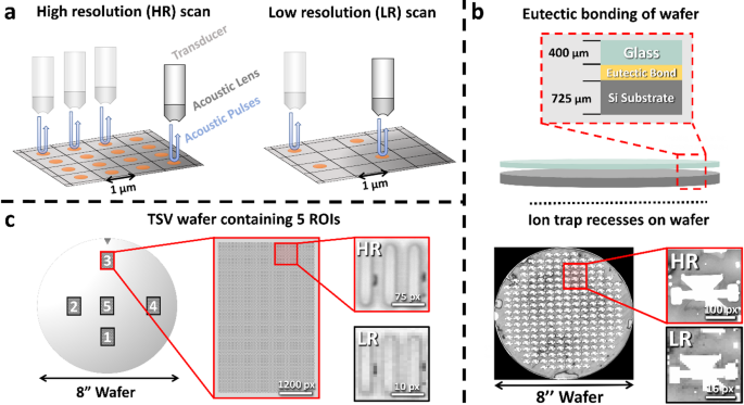
Scanning principle of a SAM and two different QC 3D integration technology specimens. (a) Scanning principle of SAM. To obtain a HR image, the transducer sends out and receives acoustic pulses at many scanning points. When using a low resolution, the transducer excites fewer pulses resulting in a shorter scanning time. (b) For the first specimen, a schematic of a bonded wafer is illustrated. A glass and unstructured silicon substrate, both fully metallized, are bonded together via eutectic bonding. A SAM C-scan image from the whole wafer containing the ion trap recesses (white grey values) is shown. Further grey values within the image can be associated with different qualities of the eutectic bond (light grey) and delamination (white and dark grey). Two magnified C-scan images for the same region of interest (ROI) are displayed on the right. They are indicated as HR and LR. (c) The second specimen shows a wafer with five TSV structures, each ROI exhibits 10,240 TSVs. The ROIs are highlighted with the numbers 1 to 5. A magnified image of ROI 3 is presented. A further zoom-in on the right highlights the TSV’s structure. HR and LR C-scan images are indicated. Winsam 8.24 software61 is employed for capturing and preprocessing the C-scan images.
Workflow—From data acquisition over image enhancement to failure analysis
The overall workflow for super resolution (SR) and the downstream image analysis is shown in Fig. 2. It consists of three stages including model selection, data acquisition and preprocessing, self-supervised learning and application of the trained SR model to resolution sensitive failure-analysis tasks, see Fig. 2a-c, respectively.
As depicted in Fig. 2a, a SR model architecture and learning strategy has to be chosen. This can be a supervised CNN like DCSCN, a SR-GAN or an iterative algorithm like InDI. Additionally, high resolution image data has to be collected by using SAM. C-scan images are then preprocessed by cropping and augmentation.
Inspired by ideas of current self-supervised real-world SR approaches50,62 the augmented HR images are then downscaled by nearest-neighbors to produce the corresponding LR counterparts. Using a simple nearest-neighbors downscaling is justified by the fact that reducing the SAM scanning resolution is physically similar to deleting every second pixel in the image. To further ensure that the downscaled LR images looks realistic, multiplicative noise has to be added, since this is a common source of degradation in acoustic microscopy39. Lastly, we also employ Gaussian blurring and WebP compression to make the architecture more resilient to other degradation mechanisms. Multiplicative noise is applied with a probability of 30% and Gaussian blur as well as compression-noise is applied with a probability of 10% to every image. Details about training parameters and datasets used are available in the Methods section.
As can be seen in Fig. 2b, we use the final LR images as input to an exemplary SR model, which outputs images with higher-resolution. Image quality can now be measured in terms of a loss function to guide the training of the exemplary model. Nevertheless, this loss function can be chosen freely and the main problem comes down to avoiding regression-to-the mean, which causes blurry and less sharp image reconstructions63.
Depending on the quality and amount of training data, the SR model can now enhance various real-world images, see Fig. 2c. The models are trained on a wide variety of C-scans, enabling them to perform well on a large range of images including different resolutions and transducer types, see Methods section for more information. The enhanced images are then used for resolution-sensitive downstream tasks like semantic segmentation or object detection, often enabling improved performance due to higher image fidelity.
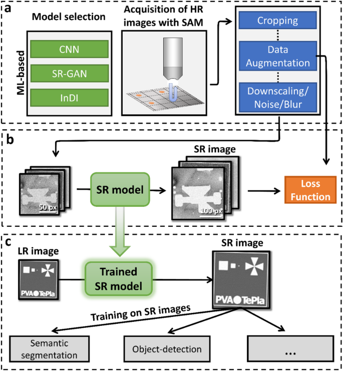
Overview of the super-resolution workflow. (a) The first step of the workflow consists out of model selection and data acquisition via SAM. The obtained C-scan images are cropped and augmented. To do self-supervised training, LR images are constructed by downscaling and altering the augmented HR images. (b) Training of the chosen model architecture utilizing the downscaled images. A predefined loss function guides the model training. (c) After training is complete, the model can be applied to enhance various other images. Further, the enhanced images can be used to improve the performance of subsequent resolution-sensitive algorithms like semantic segmentation or object-detection. Winsam 8.24 software61 is employed for capturing and preprocessing the C-scan images.
Model selection and validation for image enhancement
For image enhancement we train various modern ML-based SR architectures and compare them to classical methods, see also Table 1. The developed image enhancement shall foster to eliminate time limitations fetched by the experimental HR scans by doubling the resolution after measurement, as shown in Fig. 3. Most importantly, the SR approach should also generalize to various scanning resolutions and transducer types. To achieve this, self-supervised model training is implemented, allowing to train on much larger dataset and improving generalizability. Moreover, the ML-models are discussed not only based on the performance gained by known metrics but also by their evaluation time per image as well as energy consumption.
One can quantify the reconstruction quality of different models by calculating common metrics like the peak signal-to-noise-ratio (PSNR) and structural similarity index measure (SSIM)63,64. Both allow a comparison to other models found in literature. However, these two metrics are sensitive to small image transformations and do not capture important image characteristics like sharp edges44,63,65. Therefore, they do not present useful objectives for measuring overall real-world performance, and we aim to introduce two new metrics which try to capture more of the physical information. The first metric is called edge correlation index (EdgeC). It uses a canny edge detection algorithm to detect edges and calculates the correlation function between the detected edges in the HR and reconstructed image. Possible values of EdgeC range from + 1 to -1, corresponding to perfect correlation or anti-correlation. Furthermore, we introduce a metric based on the scale-invariant feature transform (SIFT) algorithm66,67. SIFT is a popular method to find congruent points in two images. We can employ this algorithm and count how many congruent points SIFT detects between both images. The higher the count, the better the reconstruction. More details about these metrics are presented in the Supplementary Note 2, Supplementary Fig. 2 and Supplementary Table 1.
Table 1 indicates the performance of bicubic and nearest neighbor upscaling in terms of the self-supervised regime, where the LR images are produced by artificially downscaling HR C-scan images. It is obvious that bicubic and nearest-neighbor upscaling perform poorly in terms of the introduced metrics. Nevertheless, when using AI-based models, there are several possibilities for selecting the loss function and training, leading to better reconstruction quality.
One common approach to achieve high-quality outputs is by the use of GANs. To test the capabilities of GAN models for the SR tasks, we implement a SR-GAN41. The generator has the same architecture as displayed in Fig. 3a and is trained with a combination of perceptual loss and adversarial loss, the latter representing the feedback from the discriminator. The discriminator itself is trained using a relativistic average loss68. As shown in Table 1 this SR-GAN approach shows better performance than classical models across all metrics.
Another way to produce high-quality images is by using an iterative algorithm. For this, we implement the recent inversion by direct iteration (InDI) diffusion-like algorithm, which uses a LR image and gradually increases its quality step by step43. As seen in Table 1 InDI performs good for artificially downscaled image data. However, InDI shows issues for the measured low resolution SAM image data, see Fig. 3b-c. There, real measurements of a wafer with test-structures, obtained with 50 μm/px and 100 μm/px resolution directly on the SAM, are shown. It is noticeable that the InDI algorithm is not able to reconstruct the straight lines in ROI-2 from the 100 μm/px image. Additionally, the InDI model hallucinates structures which are not there in the real HR image, as can be seen close to the edges of the cross in ROI-1. This further underscores the importance for real-world evaluations, especially for highly generative and iterative models like InDI. In fact, the problem of hallucinations in highly generative models is gaining increasing attention in the last years51,52. Similar comparisons on real-world data using the SR-GAN model can be found in Supplementary Note 3 and Supplementary Fig. 3.
Perceptual loss functions46 are another common way to produce high-quality outputs in SR tasks. We chose to implement such a perceptual loss function, employing a feature extraction neural network for extracting important features and structure from the image. The mean-averaged-error (MAE) is then calculated between those extracted features, see Method section for further details. With this loss function, the state-of-the-art SRResNet (Super Resolution Residual Network)40 is implemented, which gives results close to SR-GAN and InDI in Table 1. However, when applied to real-world data, the SRResNet performs only slightly better than bicubic upscaling, as demonstrated in Supplementary Fig. 3.
Last but not least, we also implement a more complex fully convolutional neural network based on an adapted DCSCN architecture42 trained with the same perceptual loss as SRResNet. The DCSCN architecture is exemplarily shown in Fig. 3b. Surprisingly, this model shows the best performance across nearly all metrics presented in Table 1, even outperforming the generative models like SR-GAN and InDI, as well as the SRResNet. Furthermore, DCSCN is superior to other methods under real-world applications, as displayed in Fig. 3c and Supplementary Fig. 3.
Table 1 also includes data for the evaluation time and energy consumption during training. To train the diffusion-like InDI and generative SR-GAN models, more powerful hardware has to be used, which also increases the energy consumption and environmental footprint by a factor of around two. Due to its larger parameter size and iterative approach, InDI also takes roughly one order of magnitude longer to reconstruct images. In fact, DCSCN seems to present the best balance between image quality, evaluation time and power consumption.
Detailed information about the SR-GAN, InDI, SRResNet and DCSCN architectures and training can be found in the Methods section, Supplementary Note 4 and Supplementary Fig. 4.
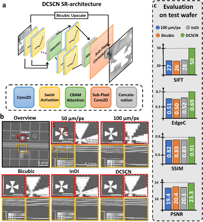
DCSCN model architecture and model evaluation of DCSCN and InDI SR. (a) Model architecture of CNN-based DCSCN SR model. The first block consists out of convolutional layers with 176, 160, 144, 128, 112, 96, 80, 64, 48 and 32 filters. The second block (reconstruction block) is split in two. It has convolutional layers with 32 and 32, 64 filters. The kernel size is 3 except for the first layers in the reconstruction block, where we use a kernel size of 1 for feature extraction. (c) Evaluation of SR on a test wafer. The upper left image shows an overview of the test structures. The colored images are zoomed in sections (ROI 1–2). ROI 1–2 are measured and displayed for different resolutions (100 μm/px and 50 μm/px). From the 100 μm/px we reconstruct a 50 μm/px image with bicubic interpolation, DCSCN and InDI. (d) PSNR, SSIM, EdgeC and the number of matched features found via a SIFT algorithm are listed as bar graphs. They show a clear advantage of the DCSCN approach compared to classical bicubic upscaling, but close to no improvement when using InDI. Winsam 8.24 software61 is employed for capturing and preprocessing the C-scan images.
Failure-analysis of a bonded ion trap wafer
To test the capabilities of SR in industrial applications, we apply the selected CNN-based DCSCN model to the eutectically bonded wafer specimen displayed in Figs. 1b and 4a. The main goal is to show how SR can decrease the time for large-scale SAM measurements and improve the accuracy of subsequent segmentation-based failure analysis.
We again note that C-scan images of the wafer with 50 μm/px and 300 μm/px resolution are available, whereas the 300 μm/px resolution is close to the resolution limit for detecting small features. Different structures, material phases and defect types are visible in the C-scan image, see also Methods section. To quantify the bond quality of the wafer, the scanned images are segmented into 3 distinct regions and the corresponding areas are evaluated, see Fig. 4a. In particular, we distinguish between ion-trap recesses (white), intact eutectic bond (blue) and delaminated eutectic bond (red). For segmentation, three separate state-of-the-art residual attention U-Net69 models, for the three different resolutions (50 μm/px, 300 μm/px and DCSCN enhanced), are trained and employed. More information on the training for the segmentation model is provided in the Methods section.
In Fig. 4b a cutout of the segmented C-scans for a resolution of 50 μm/px, 300 μm/px as well as the DCSCN-enhance image are presented. Clearly, deviations between all images can be depicted, especially between the 300 μm/px and 50 μm/px images. In hard to segment areas, like for the upper ion-trap recess in Fig. 4b, the U-Net segmentation model trained on the 300 μm/px image struggles to detect the whole ion-trap structure. In comparison, even though the DCSCN enhanced image seems to be smoothened and loses some details in comparison to the 50 μm/px image, it is obvious that there is a better qualitative correspondence and all key features are properly segmented in this case.
Figure 4c provides a quantitative comparison of the relative errors in segmented areas between the 50 μm/px, 300 μm/px, DCSCN-enhanced image and a manually labeled ground truth. When applying the DCSCN model to the 300 μm/px image, a decrease of the relative error by at least 10% or more can be established. There are three main reasons for the observed improvement. First, the LR 300 μm/px image is pixelated, leading to lower-details in fine structure and, therefore, a different area of the phases. Second, manual labeling of the LR image for subsequent training of the U-Net is more difficult due to the decreased edge-contrast, making it harder to accurately train the model. Third, when a model is trained with LR data, it has a lower amount of pixel-data to be trained with. For example, the 300 μm/px image has 36 times less pixels then the 50 μm/px image, decreasing model performance and generalizability. All these three factors can be improved by applying super-resolution before manual labeling and model training. Also, according to this reasoning, the provided findings are general and carry over to different model architectures as presented in the Supplementary Note 5 and Supplementary Table 2.
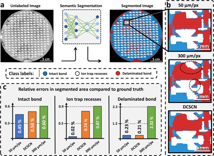
Bond quality evaluation of an eutectically bonded ion trap wafer. (a) Demonstration of ML-based segmentation using a residual attention U-Net. Three classes are distinguished: ion-trap recesses (white), intact eutectic bond (blue) and delaminated/incomplete bond (red). (b) Magnified area of the segmented wafer with a resolution of 50 μm/px, 300 μm/px and an image illustrating 300 μm/px with the applied DCSCN model, from top to bottom. Significant deviations of the 300 μm/px image from the 50 μm/px image are indicated by dashed black circles. Clearly the DCSCN and 50 μm/px images indicate higher similarity. (c) Relative errors in various segmented phases when compared to the manually labeled ground truth for the 50 μm/px, 300 μm/px and DCSCN-enhanced image. Winsam 8.24 software61 is employed for capturing and preprocessing the C-scan images.
Fast object detection and super-resolution for through-silicon-vias (TSVs)
For the failure analysis of thousands of TSVs, we localize and classify every individual TSV on the wafer, see also Fig. 1c. We implement and compare different ML-based object detection algorithms including YOLOv270 and YOLOv1271. YOLO is a so-called one-shot method, since it localizes and classifies all objects in an image within one evaluation of the neural network. This makes the method very time efficient, especially for large images.
Figure 5a shows the basic steps of the failure analysis workflow. The workflow starts by applying SR to the input image to double its size, then dividing it into a grid of cells. For YOLOv2, cells with a size of 32 × 32 pixels are usually used. For every grid cell, a neural-network then predicts three values namely, (1) a confidence score, which measures the probability of an object being present in the cell, (2) the bounding box coordinates of the object and (3) its class labels. Finally, non-maximum suppression (NMS) is used to filter out overlapping boxes with low confidence score and a statistical evaluation can be carried out.
In Fig. 5b three quality classes for the TSVs are defined. The first class contains fully intact TSVs without any sort of defect or other imperfection. The second class defines defective TSVs. This category is characterized by black or white imperfections around the edges of the TSV. The third class covers TSVs where a failure cannot be ruled out completely, e.g. they are prone to be impacted in functionality. These TSVs have a defect close to their boundary, however, the defect does not touch the TSV itself.
As a matter of fact, detecting small objects, like the TSVs shown in Fig. 5, displays critical problem for every object-detection algorithm59. Table 2 shows that all tested object detection algorithms show increased performance when trained and evaluated on the DCSCN-enhanced SR images and perform worse when trained and evaluated on the original LR images. The YOLOv2 algorithm is not even able to converge to a proper state, since its cell size is 32 × 32 pixels, limiting the model to only distinguish between objects with a minimum distance of 32 pixels. However, the TSVs illustrated in the C-scan image data have a distance of 25 px, therefore, being too close for YOLOv2 to distinguish. In contrast to this, YOLOv12, which uses multi-scale training and smaller cell sizes, is still able to localize and classify TSVs on the LR images, however, with reduced accuracy. In fact, detection accuracy for both, YOLOv2 and YOLOv12, reaches 99.8% on the SR images. This means, that only 2 out of one thousand TSVs are not detected.
The classification accuracy for sorting the TSVs into the three classes defined in Fig. 5b is evaluated to be around 96% for all models trained on the SR images, and thus close to the capabilities of the approach presented in34, however with higher time efficiency. For example, the evaluation of 10,240 TSVs takes only around 8 s for YOLOv2. To further emphasize the time-efficiency of the YOLO model, we compare it to the recently introduced end-to-end sliding window approach34 by applying it to the data provided in34, see Supplementary Note 6 and Supplementary Fig. 5. Note that the presented YOLOv2-based model architecture outperforms, in terms of time, the mentioned end-to-end sliding window approach34 by a factor of 60.
Table 2 also includes a transformer based Real-Time Detection Transformer (RT-DETR) object-detection model56. Even though this model performs good for the SR images, it underperforms in terms of detection accuracy compared to YOLOv12 on the original LR images. Also, since RT-DETR is transformer-based, model inference can only be applied on images of the same size as the training images. This is a drastic practical shortcoming since object-detection is often trained on small image crops and then applied to larger images. See the Methods section for more details.
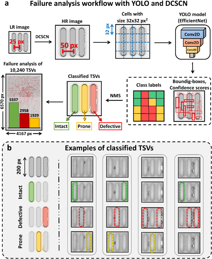
Workflow to enable YOLO object detection with SR and definition of defect labeling. (a) YOLOv2 object detection pipeline. We start by increasing the resolution of the LR scanned image by 2 times, to increase the distance between adjacent TSVs. After that, the HR image is divided into cells of 32 × 32 pixels and evaluated by the YOLO model. The YOLO model utilizes an EfficientNetV2-B0 backbone. The outputs of the model are class labels, bounding boxes and confidence scores for every grid cell. In a last step, NMS is used to filter out intersecting boxes with low confidence. This algorithm can now be used to carry out large scale failure analysis as shown for a ROI containing 10,240 TSVs. (b) TSV classification and measurements. We sort TSVs in three classes: Intact TSVs (green), defective TSVs (red) and TSVs which are prone to be impacted in functionality due to nearby defects (yellow). Winsam 8.24 software61 is employed for capturing and preprocessing the C-scan images.