The DRIVES study began participant enrollment in 2014. The primary wave of participants was referred to from the longitudinal Memory and Aging Project (Estd. 1979) and the Knight Alzheimer’s Disease Research Center (Estd. 1984)25. Additional participants were recruited from the greater Missouri-Illinois community via snowball-sampling, referral, registries, and community dissemination. The enrollment criteria required participants be: (1) cognitively normal at baseline as indicated by a Clinical Dementia Rating (CDR) of 0, (2) age 65 or older, (3) drove at least once a week, (4) had a valid and current driver’s license, (5) drove a non-adapted vehicle, and (6) consented to clinical, neuropsychological, and biomarkers collection.
All procedures involving human participants were performed in strict accordance with the ethical standards of the 1964 Declaration of Helsinki. Before any study procedures were initiated, every participant received a detailed written and verbal explanation of the study’s purpose, procedures, potential risks and benefits, data protection safeguards, research data sharing, and their right to withdraw without repercussions. Those who agreed to participate signed a written informed consent form; a copy was given to each participant, and a second copy was filed in the study records. For participants with mild cognitive impairment, written permission was obtained from their identified, legally authorized representative. The Washington University Institutional Review Board approved all informed consent and study protocols (IRBs# 201706043, 202010214, 202003209).
For this data descriptor, we chose to include only a subset of participants who were enrolled in the DRIVES Project from March 2023 to May 2023. Table 1 details the demographic breakdown of the participants collected during this time period.
DRIVES Chip
Each DRIVES datalogger, or colloquially referred to as a ‘chip,’ was installed via the onboard diagnostic port (OBD-II) of a vehicle, typically located underneath the dashboard or in the center console of a vehicle’s cabin. Internal combustion engines and hybrid vehicles manufactured from 1996 onward had to have an OBD-II port in the US; however, it could also be installed in electric vehicles using an aftermarket splitter to collect the same metrics. Chips were equipped with jamming detection, Bluetooth, a 56-channel GPS receiver with a 4-Hertz acquisition rate, and a tri-axial (X, Y, Z) accelerometer that detected changes in acceleration over +/− 16 g-force with a reporting rate of 24 Hertz, and a tri-axial gyroscope with a reporting rate of 24 Hertz. Data were collected from when the ignition was turned on until it was turned off. Within one minute after installation, the chip accesses available satellites for orientation and synchronization and begins transmitting data using cell phone towers to cloud servers supported by the vendor. The chips collected large volumes of data from participants’ vehicles while being inexpensive, reliable, and requiring no extensive modification to their vehicles. The data provided encompassed spatial, temporal, and performance metrics about the general usage of a participant’s vehicle, including the vehicle speed, a trip’s duration, and the vehicle’s lateral acceleration. These metrics were then transmitted from the chip to the commercial vendor’s back-end servers via cellphone towers, further processed, and uploaded to an Amazon Web Services (AWS) server that the project accesses for download and then additionally processed. The results of participants’ driving behavior were collected, collated, and packaged daily.
The DRIVES pipeline combined a modified commercial GPS solution (Azuga G3 Tracking DeviceTM, https://www.azuga.com/) used in fleet management in combination with custom software code to extract naturalistic driving (ND) behavior, model participants’ driving patterns, and evaluate the environments in which they drive, using Global Positioning System (GPS) and geographic information system (GIS). If a participant had more than one vehicle, they were provided with multiple chips for each vehicle to ensure comprehensive data collection across all vehicles.
Driver identification
A Bluetooth beacon, paired with the DRIVES chip, was issued to participants to address those who shared a vehicle with a family member or friend. The participant’s trips were marked with the beacon serial number, differentiating the enrolled participant’s data from other drivers. Prior to 2016, the project issued the BLE 4.0 model to a subset of participants, which had the drawbacks of questionable functionality and a shorter average battery life. From 2017 onwards, the project issued the BLE 5.0 model, which offered a longer battery life and added detection functionality.
Low-frequency data
The first set of data that the DRIVES Project processed was LFD. This data was uploaded to an AWS Simple Storage Service (S3) in 30-second intervals from a vehicle’s chip and contained periodic data (breadcrumbs) and a trip summary at the end of each vehicle trip. For every 30 seconds during a trip, the periodic data captured (1) the Coordinated Universal Time (UTC) timestamp, (2) the GPS location of the vehicle (latitude and longitude), (3) GPS heading and altitude, (4) the speed of the vehicle, and (5) the odometer readings for the vehicle while in operation. When a vehicle was not in motion, a ‘heartbeat message’ with the date, time stamp, and location was reported every three hours. The trip summary that accompanied the periodic data consisted of (1) the start location and time of a trip, (2) the end location and time of a trip, (3) the total distance traveled, (4) the total fuel consumed, and (5) a count of all hard braking, acceleration, and speeding events. After the data had been uploaded to AWS S3, it was enhanced to provide geo-coded addresses, the posted speed limit of the vehicle for each breadcrumb location, a generated trip number that auto-incremented when a new trip was started by a vehicle, and the cumulative distance measured per trip.
The driving metrics obtained from the DRIVES chip were uploaded into four separate comma-separated value (CSV) files into the AWS S3 repository. The first file, a breadcrumb report, contained all the periodic information. The second file, an activity report, provided detailed trip information by breaking down fuel usage, speed in miles per hour, number of stops, distance traveled, and driving behavior (i.e., hard-braking, speeding, idling, sudden acceleration) for each vehicle. Each trip within this file was matched to an internal participant ID using the unique ID of the installed chip and the beacon ID, if available. The third file, an events report, provided detailed information on all adverse events (i.e., hard braking, hard acceleration, speeding) at a vehicle level per trip. A hard braking event was triggered when the vehicle was moving at a speed greater than 12 miles per hour (mph), followed by a decrease in speed at the rate of eight to 12 mph per second; if the change in speed exceeded 12 mph, then the event was categorized as a hardcore braking event. A sudden acceleration event was triggered when a vehicle moving at a speed of more than three mph showed an increase in speed above the rate of eight mph per second. The last file was a summary report aggregating all daily trips carried out by each vehicle. This reported the data across the entire fleet based on drive time, idle time, stop time, miles driven, number of stops, hard braking, and sudden acceleration incidents aggregated at a daily level. In addition to these files, a vehicle inventory report, a device inventory report, and a firmware report were also provided, listing the details and status of all vehicles and chips used in the DRIVES project.
The increasing number of participants driving with their chips necessitated tracking the total number of breadcrumbs obtained daily and the status of these chips for the duration of the participants’ enrollment in the project. The DRIVES Project used a scheduler to automatically run an R script that created a daily report for the project; this report was produced every morning and sent to study personnel for monitoring. The daily report included a summary of the newly activated and offline chips with missing data. Chips could go offline for various reasons, including the vehicle having low battery voltage, being damaged in an impact event (i.e., motor vehicle crash), or being accidentally removed and not replaced by mechanics. This report also contains the number of breadcrumbs downloaded daily. The report’s summary listed breadcrumbs reported daily, and the number of chips that had trips on the given date was listed. Additionally, it also indicated the number of new chips that needed to be added to the dictionary and the number of vehicles reporting no movement. The number of vehicles with breadcrumbs not tracking at 30-second intervals (i.e., intervals > 30 s). For chips that needed to be added to, removed from, or commented on in the daily report, the DRIVES Project implemented R Shiny applications that allowed project members to modify the report as needed; the report was then updated and redistributed daily. The report was generated on a three-day lag, so the reported updates were from three days prior to allow time for a device to synchronize and re-send data if it had been driven in an area without signal coverage or no movement over a weekend.
High frequency data
Beginning in September 2022, the vendor’s telematic pipeline was upgraded to collect HFD, taking advantage of the 5G broadband network and Transmission Control Protocol (TCP) in addition to the LFD. These data were collected at periodic 1-second intervals (1Hz) along with the accelerometer and gyroscope collecting data at 24 Hz. Unlike the LFD, all driving measurements about a trip were uploaded as a single JSON file to the AWS S3 repository daily. Rather than holding an aggregate of all trips taken on a given day, each JSON file corresponded to all driving behavior measurements for a single trip taken by a single vehicle. This resulted in thousands of JSON files uploaded to the S3 repository daily, each corresponding to a trip that one of the enrolled participants drove. Each JSON file contained all periodic data and the trip start and end messages. Further, speed and revolutions per minute (RPM) data at 1 Hz from the HFD data were used to develop ‘jerk’ metrics. Counts of ‘jerk’ or change in acceleration (based on speed and RPM) were measured in different buckets. Similarly, acceleration in the X-axis was also used to develop jerk metrics using data aggregated at 0.5 seconds. A 24 Hz, Z-axis gyroscope values were aggregated at a 1-second interval to identify different turn maneuvers. A cut-off threshold of 5 degrees per second was used to show the start of a turn maneuver. A set of sequential observations that met this threshold was identified as a single turn event and summarized in a table. Both left and right turn maneuvers were identified, and corresponding fields included location, duration, and the overall degree of the maneuver for each event. Event messages were not provided in the JSON file and needed to be matched through a separate processing pipeline.
Environmental data
In addition to capturing naturalistic driving behavior, the DRIVES Project also collected latitude and longitude data, which served as a proxy for determining relationships with the sociodemographic characteristics of a participant’s neighborhood and each trip they completed. While there were numerous measures of structural and social determinants of health (S/SDOH)26, limited composite indices have not been validated nationally across the population to capture the multidimensional layers of S/SDOH. Recent research indicates that environmental factors measured by the area deprivation index (ADI) and social vulnerability index (SVI) are essential but underutilized variables when studying dementia27,28,29. We included the following: (1) the ADI rankings based on each participant’s self-reported, primary home address, (2) variables relating to the SVI of a participant’s neighborhood, (3) the weather conditions at the beginning and end of each trip, and (4) the road characteristics underlying each participant’s trip. The ADI and SVI could be obtained for any unique location throughout any trip.
To measure neighborhood-level deprivation, the DRIVES Project used both the national and state ADI rankings for participants’ recorded home addresses, using the neighborhood atlas provided by the Center for Health Disparities Research at the University of Wisconsin, Madison30,31. The DRIVES Project used the participants’ self-reported home addresses to generate geographic identifiers (geoids) using Geocode.io. Once generated, the city, state, county, and census block group numbers were combined to create a 12-digit Federal Information Processing Standards (FIPS) code that was then used to extract the national and state ADI rankings from the neighborhood atlas.
To measure county-level deprivation, the DRIVES Project used a similar procedure to extract the rankings for each participant’s neighborhood. The Centers for Disease Control and Prevention (CDC) provided the 2022 SVI percentile rankings. Similar to how the ADI rankings were extracted, the DRIVES Project used geoids corresponding to participants’ primary home addresses to create 11-digit FIPS codes; the FIPS codes were then used to extract SVI features from the 2022 SVI dataset provided by the CDC.
The DRIVES Project utilized an online historical weather and climate database, Meteostat, which contains data from thousands of weather stations and locations worldwide32. Meteostat contained an associated Python module that allowed users to connect to the database via an API. This module provided weather conditions (i.e., average temperature, precipitation, etc.) using the date and GPS coordinate values pertaining to a specific trip that connected to each participant’s trip.
Lastly, the DRIVES Project used OpenStreetMap (OSM) to capture the road characteristics underlying each participant’s trip. Using Python’s OSMnx33 and Mappymatch34 modules, the DRIVES Project extracted these characteristics as features for the pipeline using the GPS latitude and longitude values provided for each trip. These characteristics included the type of roads that participants drove on (i.e., residential or motorway), the number of intersections and dead ends, and the free-flow travel time on each road segment.
Data processing
The DRIVES Project processed the LFD and HFD in two separate pipelines, resulting in two sets of data tables for each type of frequency data. Each pipeline consisted of an ensemble of Python and R scripts that copied these files from the S3 repository onto a local project server, processed these files to enhance the data signal further, and subsequently stored the processed data tables in a popular, open-source relational database management system known as MariaDB that is made by the original developers of MySQL. Utilizing this database enabled the project to enforce relational schemas connecting all processed data tables (see Fig. 1). Both the data and the pipeline were constructed to implement the DRIVES Project’s adaptation of Fuller’s task capacity diagram (see Fig. 2), as elaborated further below. A brief outline of the processing pipeline that the DRIVES Project implements for the LFD and HFD is as follows:

An Overview of the ETL Pipeline Built for the DRIVES Project. The DRIVES Project’s data pipeline for both the LFD and HFD. Driving data captured from enrolled participants is uploaded to both the cloud (AWS S3) and external sources (e.g., REDCap, Compute resources). These data are processed with Python scripts, and outputs are stored in MariaDB for subsequent analyses.

A diagram for the DRIVES Project’s implementation of the task-capacity dyadic relationship and adaptation of Fuller’s Task-Capacity Framework (Fuller, R. (2005). Towards a general theory of driver behaviour. Accident; Analysis and Prevention, 37(3), 461–472.). Cognitive decline occurs when the task demand (TD) for driving exceeds the participant’s capacity for driving (C). Driving capacity (C) consists of a participant’s driving behavior (D) and their environmental context (E).
Data download
The first step of the pipeline involved downloading the raw data files from Azuga’s AWS S3 repository onto a local Linux storage provided by Washington University. At the end of each day, the chips installed in participants’ vehicles sent all recorded spatial, temporal, and performance metrics to Azuga’s backend servers. These chips had a 3-day lag built in for transmitting the data to these servers. Therefore, all newly transmitted metrics for a given day were obtained from the participants’ vehicles three days prior. Once Azuga obtained the data, they used their internal pipelines to further process these metrics into two data formats: tabular format in the form of CSV files for the LFD and document format in the form of JSON files for the HFD. The following morning, the DRIVES Project used a Python script to synchronize its local RIS storage with the AWS S3 repository containing the raw data files. This script used the boto3 module, which established a Hypertext Transfer Protocol Secure (HTTPS) connection between the local storage and the AWS S3 repository. Once synchronized, the script compared the files on the S3 repository and the files on the RIS storage; all newly added files to the S3 repository were downloaded onto the local storage. To ensure that the appropriate number of data files were downloaded daily, the DRIVES Project implemented a separate Python script that (1) created a logfile that detailed the CSV files that the pipeline downloaded for the LFD and (2) tallied the number of JSON files that were downloaded for HFD and emailed this number to the project team members. If there were missing CSV files or if quality control was not performed, and the number of JSON files fell below a threshold of 1000, the pipeline sent the project team an email notifying them of the insufficient files. The pipeline continued onto data processing if there were files present. If no files were present on the local storage for either the LFD or HFD, the pipeline automatically halted, and its associated Python script wrote to a log file detailing the lack of files to process.
Data processing
Upon downloading the raw files, the DRIVES Project executed two Python scripts that processed the LFD and HFD separately. Both scripts shared the same purpose: to convert their respective input data into a more interpretable and tabular format that could be stored and used for data analysis.
Since the raw data had already been downloaded in tabular format, processing the LFD was simple for the DRIVES Project. There were a total of four CSV files to process for the LFD, each file holding information measured for all trips taken across all vehicles on a given day. These files were (1) the breadcrumbs file that contained periodic driving data that the chips recorded, (2) an activity file that contained all activity events during a trip (i.e., hard braking and acceleration), (3) an events file that contained any information relating to an impact event(s) experienced by the vehicle, and (4) a summary file that contained an aggregation of trips carried out in a day by each vehicle. The DRIVES Project used Python’s pandas module to create four separate data frames using the information from each CSV file. Each trip within these data frames was then mapped to a participant using its vehicle ID and beacon ID information that was available in Research Electronic Data Capture (REDCap); if a participant was not issued a beacon, the trip data was only mapped to the vehicle ID. Each trip was also assigned a week number for the week that the trip occurred in; the weeks were numbered continuously starting from January 1st, 2015. For each data frame, the DRIVES Project transformed its included features as needed for later analyses. These transformations involved utilizing the datetime module to convert the local time of each trip to coordinated universal time (UTC), calculating the week number and month from the trip start time, and using the suntime module to calculate both the sunset and sunrise times in UTC using the local time of the trip. During data processing, the DRIVES Project used Python’s logging module to write all processing steps and potential errors to a logfile that the project team could use to track the script’s efficiency. If any one trip was missing data, all data collected for that trip was excluded from the processing pipeline and written to the logfile for the project team members to review (see Technical Validation, Missing data). The result of the LFD processing was four data frames, each containing the processed data for one of the four raw CSV files. Lastly, the DRIVES Project used Python’s MariaDB module to connect to a database in MariaDB and store these data frames for downstream analyses.
Unlike the LFD, the raw HFD were stored in a document format JSON files. These JSON files were generated for each trip taken by each participant’s vehicle, resulting in thousands of JSON files downloaded onto the RIS storage on a given day. Unlike with the LFD, each JSON file also contained all the GPS, events, and trip summary measurements in a single file. Because these measurements were collected at 24 Hz per second, the files were larger and more granular than the raw data files downloaded for the LFD. In addition to the measurements mentioned above, these files also held the recorded vehicle’s acceleration that was measured by both the accelerometer and the gyroscope across all 24 Hz for the duration of the trip. Like the LFD, the DRIVES Project implemented a Python script that processed each trip JSON file, built a data table having all trip measurements obtained across all vehicles for a given day, and uploaded that table to MariaDB for further analyses. Since the raw data was processed in document format, this script incorporated more thorough transformation methodologies with the data. These methods included converting the local time of the trip to UTC, transforming the accelerometer and gyroscope acceleration measurements from radians to degrees, and adjusting vehicle speed to account for gravitational forces. Like the LFD, this script also wrote all processing steps and potential errors to a logfile that the project team could use to review the processing for any given day. If a trip JSON file was missing data, the script stopped processing it and wrote it to a logfile for the project team to review (see Technical Validation, Missing data). When all JSON files had been processed, the script pulled all the processed measurements into a single data table, which was then pushed to MariaDB.
Data postprocessing
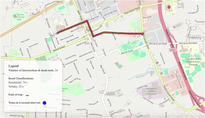
Once the LFD and HFD had been processed and uploaded to MariaDB, the DRIVES Project implemented a script that performed postprocessing on both datasets to create additional data tables in MariaDB. A subset of these tables included multiple aggregates of the naturalistic driving ND data at the weekly and monthly level; the DRIVES Project used pandas in conjunction with each trip’s assigned week number and start date to create the weekly and monthly aggregated data tables. Another subset of these added tables included specific tables that contained additional metrics for the LFD and HFD separately. For the LFD, the project incorporated a Python script that computed metrics for each overspeeding event where a participant drove above the speed limit in a particular area. At the trip-level, this script used a combination of Python’s NumPy and datetime modules to compute the time at which each speeding event occurred, the average speed during the event, and the difference between the vehicle’s speed and the speed limit in each area. The script later aggregated these speeding events to obtain the total count of events for a given day. To validate the quality of the driving metrics obtained from the LFD, we create kernel density estimates for a subset of vehicles within a specified timeframe. For example, in Fig. 3, a kernel density estimate was created for the maximum speed, average speed, total trip time, and total distance travelled across three vehicles during the Spring of 2023. For the HFD, the project used a Python script to compute the jerk events and turn maneuvers experienced by the participants during each trip. Since the HFD was captured at 1 Hz per second, the pipeline could use the vehicle speed, engine RPM, and acceleration as measured by the accelerometer to compute all jerk events experienced by a vehicle during each trip. For turn maneuvers, the script used an in-lab custom module to compute the total number of turns a participant took during a trip. The module did this by combining a vehicle’s speed, acceleration as measured by its gyroscope, and GPS coordinates. Lastly, the script also calculated the mobility metrics for each vehicle, both at the weekly and monthly aggregate levels. The script utilized Python’s scikit-mobility35 module to compute metrics such as the maximum distance a participant traveled from an estimated home address using “skmob.measures.individual.max_distance_from_home()”, the unique destinations traveled to with “skmob.measures.individual.number_of_locations()”, and the total entropy of a participant’s vehicle by “skmob.measures.individual.real_entropy()”. These metrics were aggregated for all trips at the weekly and monthly levels and then stored in separate data tables. Once the postprocessing was completed, new data tables were created to hold the aggregated data and stored as separate tables on MariaDB. At the end of both pipelines, a Python script was used to extract the sociodemographic features from their sources and add them as features to both the LFD and HFD data tables. The ADI national and state rankings were extracted using the 12-digit FIPS code associated with each participant’s self-reported home address. Like the ADI rankings, the SVI features provided by the CDC were extracted by using the 11-digit FIPS code associated with each participant’s home address. The ADI and SVI features were then merged into the LFD and HFD tables using the participant ID associated with each participant’s home address. By incorporating these sociodemographic features, a comparison can be made regarding various driving metrics across different neighborhoods contingent upon their deprivation status. Examples of such metrics include the average vehicle speed and the frequency of overspeeding incidents among our participants categorized by neighborhood status (refer to Figs. 4,5, respectively). In addition to these features, the weather conditions at the beginning and end of each trip were computed using the Meteostat module. The script provided the Meteostat API with the start- and end-of-trip GPS coordinates and time values. As a result, the API provided the average temperature, humidity, precipitation, and wind speed throughout the duration of a trip. With the features from Meteostat, we can observe the fluctuations in the average temperature during our participants’ trips over time. For example, in Fig. 6, we are able to measure the average temperature across the trips for five participants throughout the Spring of 2023. Lastly, the script used Python’s OSMnx module to get the underlying road conditions that each participant drove in. The script provided the GPS coordinates and time recorded throughout a trip as input parameters for the module; in turn, OSMnx provided the road conditions experienced by the vehicle during the trip, such as the smoothness of the road, the traffic flow, and the number of intersections within a route. Figures 7–9 detail the GPS routes taken by three of our participants within the St. Louis area.
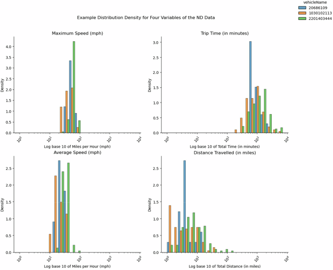
An Example Distribution Density for Four Driving Metrics. A facet plot contains four density distributions for four naturalistic driving features; these features are captured in both the LFD and HFD datasets. Displayed are the density distributions for maximum speeds (mph), the total trip times (in minutes), the average speeds (mph), and the total distance traveled (in miles) for all trips taken by three vehicles in the 2023 calendar year.

The Average Speed by Neighborhood based on the Area Deprivation Index. Area Deprivation Index (ADI) of participants’ homes and average speeding between participants ranked across quintiles. One-way ANOVA of participants based on their mean speed for all trips taken in 2023. Participants are divided into quintiles based on the ADI rankings of their primary home addresses.
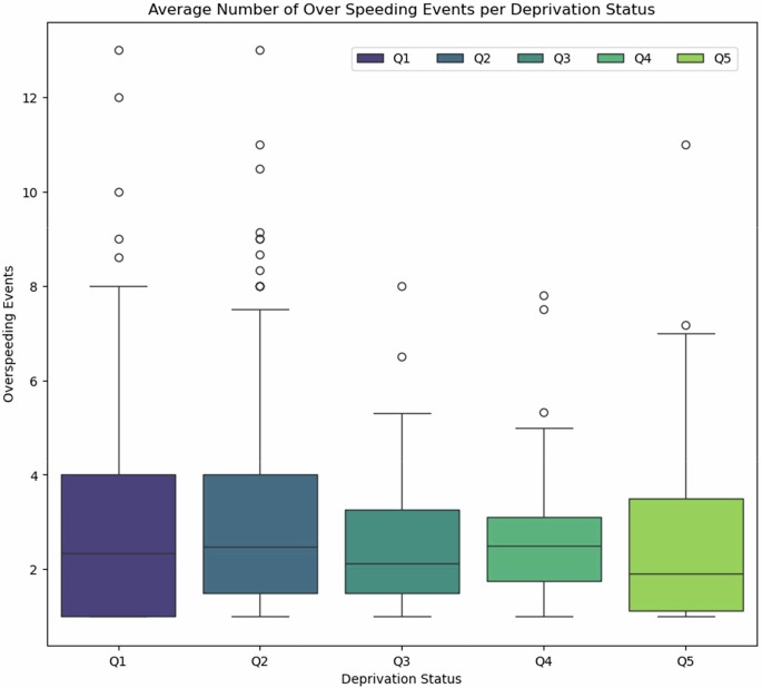
Total Number of Overspeeding Events by Neighborhood based on Social Vulnerability Index. A visualization of the difference in recorded overspeeding events between participants ranked in different quintiles using the Social Vulnerability Index (SVI) as a proxy for deprivation. Demonstrates how participants’ environment influences driving behavior.

Average Temperature Across All Trips Taken in Spring 2023. The DRIVES Project leverages the Meteostat module to capture contextual weather conditions, such as average temperature, for trips taken by participants using trip date and GPS coordinates. The project gains insights into how weather affects participants’ driving behavior over time by modeling average temperatures and their influence on driving frequency and duration.

OSMnx Map of an Urban Trip.

OSMnx Map of a Suburban Trip.
OSMnx Map of a Rural Trip.