In this section, we review the theoretical tools used to compute the three-dimensional phase diagram. We follow ref. 31 closely and elaborate in detail when needed. We mainly focus on the disordered side of the FE transition and comment on how we extend the analysis to the ordered side.
Self-energies
We start with the bosonic and fermionic self-energies, which are computed to one-loop order. The bosonic self-energy is obtained following the one-loop fermionic bubble as shown diagrammatically in Fig. 6a. Following ref. 31, we construct a vector basis and assign three orthonormal vectors corresponding to each vector k as \({\hat{k}}_{t}\), \({\hat{k}}_{u}\), \(\hat{k}\), as shown in Fig. 6b. We define \({\hat{k}}_{t}\) as \({\hat{k}}_{t}=\hat{z}\times \hat{k}/| \hat{z}\times \hat{k}|\) to ensure it lies in the xy plane. We then choose \({\hat{k}}_{u}\) as \({\hat{k}}_{u}={\hat{k}}_{t}\times \hat{k}\), such that its projection on the xy plane is parallel to the projection of \(\hat{k}\) on the same plane. Expressing the form-factor in Eq. (5) in the new coordinate space, we obtain
$$\hat{k}\times {\boldsymbol{\sigma }}\to {\hat{k}}_{t}\left(\sin \theta {\sigma }_{x}-\cos \theta {\sigma }_{y}\right)-{\hat{k}}_{u}{\sigma }_{z}\,.$$
(22)
where θ is the polar angle. The polarization bubble assumes the form
$$\begin{array}{lll}\hat{\Pi }(q)=\displaystyle\frac{\bar{g}}{{k}_{a}^{3}}T\,\,\text{Tr}\,\mathop{\sum}\limits_{k}\left({\hat{k}}_{t}\left(\sin \theta {\sigma }_{x}-\cos \theta {\sigma }_{y}\right)-{\hat{k}}_{u}{\sigma }_{z}\right)\\\qquad\quad\,\, \times \left[G(k+q/2)G(k-q/2)\right]\left({\hat{k}}_{t}\left(\sin \theta {\sigma }_{x}-\cos \theta {\sigma }_{y}\right)-{\hat{k}}_{u}{\sigma }_{z}\right)\\\qquad\,\,=\displaystyle\frac{\bar{g}}{{k}_{a}^{3}}T\,\mathop{\sum}\limits_{k}G(k+q/2)G(k-q/2)\left({\hat{k}}_{t}{\hat{k}}_{t}+{\hat{k}}_{u}{\hat{k}}_{u}\right)\,,\end{array}$$
(23)
where G(k) is the fermionic propagator. The fermionic and bosonic four-vectors are denoted by k = (k0, k) and q = (q0, q), respectively, with k0 and q0 representing Matsubara frequencies, and k and q representing 3D momentum. The trace in the first step in Eq. (23) is over spin indices. The second step is obtained by following spin summations.
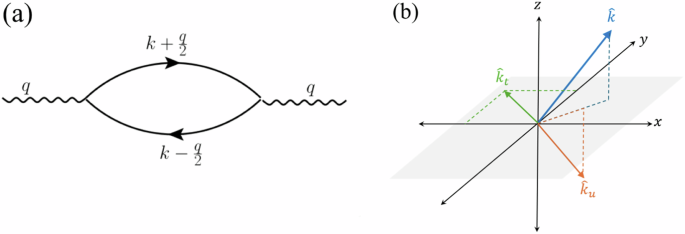
a The diagram of the one-loop polarization bubble. The curvy lines represent the boson propagator, and the straight lines with the arrow represent the electronic Green’s function. b The basis for describing the transverse mode. The components transverse to \(\hat{k}\) are \({\hat{k}}_{t}\) and \({\hat{k}}_{u}\).
The bubble can then be parameterized as
$$\hat{\Pi }(q)=\Pi (q)\hat{P}(\hat{q})\,,$$
(24)
where \(\hat{P}(\hat{q})\) is the projector onto the plane transverse to q. The magnitude of the bubble Π(q), is then given by
$$\begin{array}{lll}\Pi (q)=\frac{\bar{g}}{{k}_{a}^{3}}T\,\mathop{\sum}\limits _{k}G(k+q/2)G(k-q/2)\\\qquad\, =\frac{\bar{g}{\nu }_{F}}{4\pi }\displaystyle\int\left(\frac{1}{({k}_{0}+{q}_{0}/2)+i{\epsilon }_{{\boldsymbol{k}}+{\boldsymbol{q}}/2}}\right)\left(\frac{1}{({k}_{0}-{q}_{0}/2)+i{\epsilon }_{{\boldsymbol{k}}-{\boldsymbol{q}}/2}}\right)\,\frac{d{k}_{0}}{2\pi }\,d{\epsilon }_{k}\,d(\cos \theta )\,d\phi \\\qquad\, =\frac{\bar{g}{\nu }_{F}}{4\pi }\displaystyle\int\frac{\left[\theta (-{\epsilon }_{{\boldsymbol{k}}})-\theta (-{\epsilon }_{{\boldsymbol{k}}+{\boldsymbol{q}}})\right]}{{v}_{F}| {\boldsymbol{q}}| \,\hat{k}\cdot \hat{q}-i{q}_{0}}\,d{\epsilon }_{k}\,d(\cos \theta )\,d\phi \\\qquad\, =\bar{g}{\nu }_{F}\left[1-\frac{| {q}_{0}| }{{v}_{F}| {\boldsymbol{q}}| }\arctan \left(\frac{{v}_{F}| {\boldsymbol{q}}| }{| {q}_{0}| }\right)\right]\,.\end{array}$$
(25)
This result gives Eq. (6). Here, we have converted from momentum to energy integration
$$\begin{array}{lll}\displaystyle\frac{\bar{g}}{{k}_{a}^{3}}\displaystyle\frac{{d}^{3}k}{{\left(2\pi \right)}^{3}}=\displaystyle\frac{\bar{g}}{4\pi }\left(\displaystyle\frac{{m}^{* }{k}_{F}}{2{\pi }^{2}{k}_{a}^{3}}\right)\left(\displaystyle\frac{k\,dk}{{m}^{* }}\right)d(\cos \theta )\,d\phi \\\\\qquad\qquad=\displaystyle\frac{\bar{g}{\nu }_{F}}{4\pi }d{\epsilon }_{k}\,d(\cos \theta )\,d\phi \,,\end{array}$$
(26)
where \({\nu }_{F}={k}_{F}^{2}/2{\pi }^{2}{v}_{F}{k}_{a}^{3}\) is the 3D density of states per spin at the Fermi level, and ka = 1/a. In the limit ∣q0∣ ≪ vF∣q∣ the polarization bubble assumes the form
$$\Pi (q)\approx \bar{g}{\nu }_{F}\left(1-\frac{\pi }{2}\frac{| {q}_{0}| }{{v}_{F}| {\boldsymbol{q}}| }\right),$$
(27)
where we have used the identity \(\left[\arctan (x)+\arctan (\frac{1}{x})\right]=\frac{\pi }{2}\). Eq. (27) is the Landau damping, which played an important role in cutting off the effectiveness of the non-linear term in pairing.
Next, we focus on the fermionic self-energy in the normal state. It is shown diagrammatically in Fig. 7. It assumes the following form after the spin summation and projection on the transverse sector.
$$\begin{array}{lll}\Sigma ({k}_{0})=\displaystyle\frac{\bar{g}}{{k}_{a}^{3}}T\mathop{\sum}\limits _{{p}_{0}}\displaystyle\int\,G(p)D(p-k)\,\displaystyle\frac{{d}^{3}p}{{(2\pi )}^{3}}\\\\\qquad\quad =\frac{\bar{g}}{{v}_{F}{k}_{a}}\frac{1}{{(2\pi )}^{3}}T\mathop{\sum}\limits _{{p}_{0}}d({p}_{0}-{k}_{0})\displaystyle\int\,d\epsilon \displaystyle\frac{1}{i{p}_{0}-\epsilon }\\\\\qquad\quad =\displaystyle\frac{-i\bar{g}{\nu }_{F}}{4{k}_{F}^{2}{a}^{2}}T\mathop{\sum}\limits _{{p}_{0}}d({p}_{0}-{k}_{0})\,\text{sgn}\,({p}_{0})\,,\end{array}$$
(28)
where we have factorized the integration over 3D momentum d3p to components parallel and transverse to the Fermi surface
$$\frac{\bar{g}}{{k}_{a}^{3}}\frac{{d}^{3}p}{{(2\pi )}^{3}}=\left(\frac{1}{{k}_{a}^{2}}\right)\frac{1}{4\pi }\frac{\bar{g}{\nu }_{F}}{{k}_{F}^{2}{a}^{2}}{d}^{2}{p}_{\parallel }d{\epsilon }_{\perp }\,.$$
(29)
Here, the momentum component parallel to the Fermi surface is denoted by p∥, and energy is denoted by ϵ⊥ = vFp⊥ with p⊥ being the momentum component perpendicular to the Fermi surface. In Eq. (28), D represents the bosonic propagator, and the function, d(Ω), of the bosonic frequency Ω = p0 −k0 is obtained by integrating the bosonic propagator D(Ω, p∥) over the momentum d2p∥ up to the Brillouin zone boundary Λ = π/a
$$\frac{1}{{k}_{a}^{2}}d(\Omega )=\mathop{\displaystyle\int}\nolimits_{0}^{\Lambda /{k}_{a}}\frac{{p}_{\parallel }d{p}_{\parallel }}{r+| {{\boldsymbol{p}}}_{\parallel }{| }^{2}+{\left(\frac{\Omega }{c{k}_{a}}\right)}^{2}+\frac{\bar{g}{\nu }_{F}| \Omega | }{{v}_{F}{k}_{a}| {{\boldsymbol{p}}}_{\parallel }| }\arctan \left(\frac{{v}_{F}{k}_{a}| {{\boldsymbol{p}}}_{\parallel }| }{| \Omega | }\right)}\,,$$
(30)
where we have used the expression for the polarization bubble in Eq. (25), renormalize r as \(r=r-\bar{g}{\nu }_{F}\), and rescale the integration variable as p∥/ka → p∥. For simplicity, we neglect the bosonic frequency term \({(\Omega /c{k}_{a})}^{2}\) in Eq. (30). Then, the bosonic function attains the following form at the QCP (r = 0) and in the limit ∣Ω∣ ≪ vF∣p∥∣.
$$\frac{1}{{k}_{a}^{2}}d(\Omega )=\mathop{\displaystyle\int}\nolimits_{0}^{\Lambda /{k}_{a}}\frac{qdq}{| {\boldsymbol{q}}{| }^{2}+\frac{\pi \bar{g}{\nu }_{F}}{2}\frac{| \Omega | }{{v}_{F}{k}_{a}| {\boldsymbol{q}}| }}=\ln {\left[1+{\left(\frac{\Lambda }{{k}_{a}}\right)}^{3}\frac{2{v}_{F}{k}_{a}}{\pi \bar{g}{\nu }_{F}| \Omega | }\right]}^{1/3}\,.$$
(31)
Inserting this into Eq. (28), we obtain an expression for the fermionic self-energy at the QCP
$$\Sigma ({k}_{0})=-i\frac{\bar{g}}{4{\pi }^{2}{v}_{F}{k}_{a}}{k}_{0}\ln {\left(\frac{{\omega }_{\Lambda }}{| {k}_{0}| }\right)}^{1/3}\,,$$
(32)
where we have defined \({\omega }_{\Lambda }=2{v}_{F}{\Lambda }^{3}/\pi \bar{g}{\nu }_{F}{k}_{a}^{2}\).
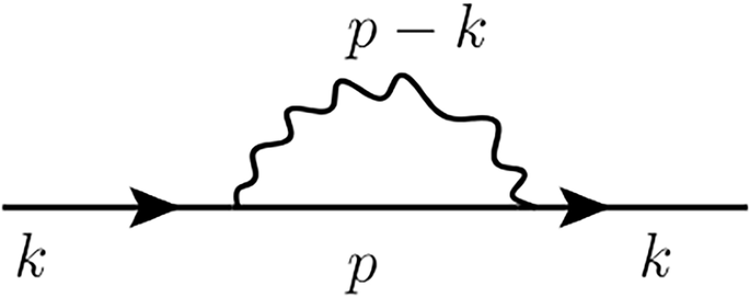
The wavy line represents the boson propagator, and the solid lines represent fermion propagators.
Gap equation
In this section, we focus on the linearized equation for the pairing vertex, shown diagrammatically in Fig. 8. It assumes the form
$${\Phi }_{\alpha \beta }(k)=\frac{\bar{g}T}{{k}_{a}^{3}}\sum _{{p}_{0}}\displaystyle\int\,\frac{{d}^{3}p}{{(2\pi )}^{3}}G(p)G(-p)D(p-k)\,{{\boldsymbol{\gamma }}}^{\nu \alpha }(-\hat{k}){\Phi }_{\nu \mu }(k)\cdot \hat{P}(\hat{q})\cdot {{\boldsymbol{\gamma }}}^{\mu \beta }(\hat{k})\,,$$
(33)
where the interaction form factor, arising due to the vector coupling, is represented by \({\boldsymbol{\gamma }}(\hat{k})=\hat{k}\times {\boldsymbol{\sigma }}\). We decompose the form factor in the vector basis \({\hat{k}}_{t}\), \({\hat{k}}_{u}\), \(\hat{k}\) as \(\gamma (\hat{k})=\hat{k}\times {\boldsymbol{\sigma }}={\sigma }_{u}{\hat{k}}_{t}-{\sigma }_{t}{\hat{k}}_{u}\), where \({\sigma }_{t}={\hat{k}}_{t}\cdot {\boldsymbol{\sigma }}\) and \({\sigma }_{u}={\hat{k}}_{u}\cdot {\boldsymbol{\sigma }}\). Since \(\hat{q}\) is approximately parallel to the FS, lying in a plane spanned by \({\hat{k}}_{u}\) and \({\hat{k}}_{t}\), we can express \(\hat{q}\) as \(\hat{q}\approx \cos \phi {\hat{k}}_{u}+\sin \phi {\hat{k}}_{t}\). Additionally, the gap function, Φ(k), can be decomposed as a sum over irreducible representations \(\Phi (k)=i{\sigma }_{y}\sum _{nj}{\phi }_{nj}({k}_{0}){F}_{n}^{j}(\hat{k})\)31. The leading attractive pairing channel in these systems is well known to be singlet14,31. For further analysis, we consider only the singlet pairing where n = 0 and \({F}_{n}^{j}=1\). We denote ϕnj at n = 0 as ϕ. The spin summations and projection on the transverse sector follow
$$\begin{array}{lll}&{\left(-\hat{k}\times {\boldsymbol{\sigma }}\right)}_{\nu \alpha }{\Phi }_{\nu \mu }({p}_{0},{\boldsymbol{k}})\cdot \hat{P}(q)\cdot {\left(\hat{k}\times {\boldsymbol{\sigma }}\right)}_{\mu \beta }\\ &=-\left(\cos \phi {\sigma }_{t}^{T}-\sin \phi {\sigma }_{u}^{T}\right)i{\sigma }_{y}\phi ({p}_{0})\left(\cos \phi {\sigma }_{t}-\sin \phi {\sigma }_{u}\right)\\ &=i{\sigma }_{y}\phi ({p}_{0})\,,\end{array}$$
(34)
where we have used the identities \({\sigma }_{j}^{T}i{\sigma }_{y}=-i{\sigma }_{y}{\sigma }_{j}\) and (σ ⋅ a)(σ ⋅ b) = (a ⋅ b)σ0 + (a × b)σ. Hence, we simplify Eq. (33) as
$$\begin{array}{lll}\phi ({k}_{0})=\frac{\bar{g}}{{v}_{F}{k}_{a}}\frac{1}{{(2\pi )}^{3}}T\mathop{\sum}\limits _{{p}_{0}}d({p}_{0}-{k}_{0})\phi ({p}_{0})\mathop{\int}\nolimits_{-\infty }^{\infty }d\epsilon \frac{1}{i\tilde{\Sigma }({p}_{0})-\epsilon }\,\frac{1}{-i\tilde{\Sigma }({p}_{0})-\epsilon }\\\\\qquad\quad=\frac{\bar{g}{\nu }_{F}{k}_{a}^{2}}{4{k}_{F}^{2}}T\mathop{\sum}\limits _{{p}_{0}}\frac{d({p}_{0}-{k}_{0})\phi ({p}_{0})}{| \tilde{\Sigma }({p}_{0})| }\,,\end{array}$$
(35)
where we have defined \(\tilde{\Sigma }({p}_{0})={p}_{0}+\Sigma ({p}_{0})\). This result is also shown in Eq. (11) where the effective coupling constant is defined as \(\lambda =\bar{g}{\nu }_{F}/4{({k}_{F}a)}^{2}\).
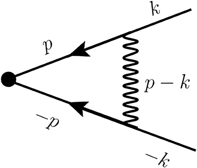
The solid and wavy lines represent the boson and fermion propagators, respectively.
Exclusion of thermal contribution from the gap equation
Both the expressions for the self-energy, Σ(k0), and the pairing vertex, ϕ(k0), as presented in Eq. (28) and Eq. (35), respectively, include terms with k0 = p0 that contribute divergently at the QCP. In the following, we discuss the procedure for discarding this divergent term. Within the framework of Eliashberg theory, the fermionic full Green’s function, \(\hat{G}\), and self-energy, \(\hat{\Sigma }\), in Nambu space, can be expressed as ref. 66
$$\begin{array}{lll}\hat{\Sigma }({k}_{0})=-i\Sigma ({k}_{0}){\hat{\tau }}_{0}-\phi ({k}_{0}){\hat{\tau }}_{1}\,,\\ {\hat{G}}^{-1}({\epsilon }_{k},{k}_{0})={\hat{G}}_{0}^{-1}({\epsilon }_{k},{k}_{0})-\hat{\Sigma }({k}_{0})=i\tilde{\Sigma }({k}_{0}){\hat{\tau }}_{0}-{\epsilon }_{k}{\hat{\tau }}_{3}+\phi ({k}_{0}){\hat{\tau }}_{1}\,.\end{array}$$
(36)
Here, \(\hat{\tau }\) are the Pauli matrices in the particle-hole space. ϵk represents the fermionic dispersion in the normal state. \({\hat{G}}_{0}\) is the Green’s function for the non-interacting fermions. ϕ(k0) is the pairing vertex, and Σ is the regular self-energy (not in Nambu space). \(\hat{\Sigma }\) can be written using \(\hat{G}\) as
$$\begin{array}{lll}\hat{\Sigma }({k}_{0})=\frac{\lambda }{\pi }T\mathop{\sum}\limits _{{p}_{0}}d({p}_{0}-{k}_{0})\displaystyle\int\,d{\epsilon }_{p}\hat{G}({p}_{0},{\epsilon }_{p})\,,\\ -i\Sigma ({k}_{0}){\hat{\tau }}_{0}-\phi ({k}_{0}){\hat{\tau }}_{1}=\frac{\lambda }{\pi }T\mathop{\sum}\limits _{{p}_{0}}d({p}_{0}-{k}_{0})\displaystyle\int\,d{\epsilon }_{p}\frac{-i\tilde{\Sigma }({p}_{0}){\hat{\tau }}_{0}-{\epsilon }_{p}{\hat{\tau }}_{3}+\phi ({p}_{0}){\hat{\tau }}_{1}}{{\tilde{\Sigma }}^{2}({p}_{0})+{\epsilon }_{p}^{2}+{\phi }^{2}({p}_{0})}\,.\end{array}$$
(37)
where λ was defined in Eq. (12). We have also decomposed the momentum into components parallel and perpendicular to the Fermi surface, as discussed in the previous section. Comparing the coefficients of the Pauli matrices in Eq. (37), we obtain the following set of Eliashberg equations.
$$\begin{array}{lll}\Sigma ({k}_{0})=\frac{\lambda }{\pi }T\mathop{\sum}\limits _{{p}_{0}}d({p}_{0}-{k}_{0})\tilde{\Sigma }({p}_{0})\int\,d{\epsilon }_{p}\frac{1}{{\tilde{\Sigma }}^{2}({p}_{0})+{\epsilon }_{p}^{2}+{\phi }^{2}({p}_{0})}\\\\\qquad\quad =\frac{\lambda }{\pi }T\mathop{\sum}\limits _{{p}_{0}}d({p}_{0}-{k}_{0})\tilde{\Sigma }({p}_{0})\frac{\pi }{\sqrt{{\tilde{\Sigma }}^{2}({p}_{0})+{\phi }^{2}({p}_{0})}}\,,\\ \phi ({k}_{0})=\frac{\lambda }{\pi }T\mathop{\sum}\limits _{{p}_{0}}d({p}_{0}-{k}_{0})\phi ({p}_{0})\frac{\pi }{\sqrt{{\tilde{\Sigma }}^{2}({p}_{0})+{\phi }^{2}({p}_{0})}}\,.\end{array}$$
(38)
The coupled Eliashberg equations for self-energy and pairing vertex are then given by refs. 66,67
$$\tilde{\Sigma }({k}_{0})={k}_{0}+\lambda T\sum _{{p}_{0}}d({p}_{0}-{k}_{0})\frac{\tilde{\Sigma }({p}_{0})}{\sqrt{{\tilde{\Sigma }}^{2}({p}_{0})+{\phi }^{2}({p}_{0})}}\,.$$
(39)
$$\phi ({k}_{0})=\lambda T\sum _{{p}_{0}}d({p}_{0}-{k}_{0})\frac{\phi ({p}_{0})}{\sqrt{{\tilde{\Sigma }}^{2}({p}_{0})+{\phi }^{2}({p}_{0})}}\,.$$
(40)
The interaction term d(p0 −k0) has a diverging contribution at k0 = p0 at the QCP (see Eq. (31)), which represents the thermal fluctuation31,35. This is similar to the effect of non-magnetic impurities and should not affect Tc according to Anderson’s theorem87. We remove the thermal contribution in the gap equation and self-energy by subtracting the term with k0 = p0 from Eq. (39) and Eq. (40) in the following manner64,65,66,67 :
$$\begin{array}{lll}{\tilde{\Sigma }}^{{\prime} }({k}_{0})=\tilde{\Sigma }({k}_{0})(1-Q({k}_{0}))\,,\\ {\phi }^{{\prime} }({k}_{0})=\phi ({k}_{0})(1-Q({k}_{0}))\,,\end{array}$$
(41)
where,
$$Q({k}_{0})=\lambda T\frac{\,d(0)}{\sqrt{{\tilde{\Sigma }}^{2}({k}_{0})+{\phi }^{2}({k}_{0})}}\,.$$
(42)
At this stage, a new gap function \(\Delta ({k}_{0})={k}_{0}\,\phi ({k}_{0})/\tilde{\Sigma }({k}_{0})\) is convenient64,65,66,67 since it is invariant under the transformation in Eq. (41) (\(\phi ({k}_{0})/\tilde{\Sigma }({k}_{0})={\phi }^{{\prime} }({k}_{0})/{\tilde{\Sigma }}^{{\prime} }({k}_{0})\)). Thus, after excluding the thermal contribution and incorporating the gap function, Δ(k0), Eq. (39) takes the form
$$\begin{array}{lll}{\tilde{\Sigma }}^{{\prime} }({k}_{0})={k}_{0}+\lambda T\mathop{\sum}\limits _{{p}_{0}\ne {k}_{0}}d({p}_{0}-{k}_{0})\frac{{p}_{0}}{\sqrt{{p}_{0}^{2}+{\Delta }^{2}({p}_{0})}}\,,\\ \frac{{\tilde{\Sigma }}^{{\prime} }({k}_{0})\Delta ({k}_{0})}{{k}_{0}}={\phi }^{{\prime} }({k}_{0})=\Delta ({k}_{0})+\lambda T\mathop{\sum}\limits _{{p}_{0}\ne {k}_{0}}d({p}_{0}-{k}_{0})\frac{\Delta ({k}_{0}){p}_{0}/{k}_{0}}{\sqrt{{p}_{0}^{2}+{\Delta }^{2}({p}_{0})}}\,.\end{array}$$
(43)
Similarly, Eq. (40) takes the form
$${\phi }^{{\prime} }({k}_{0})=\lambda T\sum _{{p}_{0}\ne {k}_{0}}d({p}_{0}-{k}_{0})\frac{\Delta ({p}_{0})}{\sqrt{{p}_{0}^{2}+{\Delta }^{2}({p}_{0})}}\,.$$
(44)
Finally, Eq. (43) and Eq. (44) lead to
$$\begin{array}{lll}\Delta ({k}_{0})=\lambda T\mathop{\sum}\limits _{{p}_{0}\ne {k}_{0}}d({p}_{0}-{k}_{0})\frac{\Delta ({p}_{0})-\Delta ({k}_{0})\frac{{p}_{0}}{{k}_{0}}}{\sqrt{{p}_{0}^{2}+{\Delta }^{2}({p}_{0})}}\\\\\qquad\quad =\lambda T\mathop{\sum}\limits _{{p}_{0} > 0,{p}_{0}\ne {k}_{0}}\frac{\Delta ({p}_{0})}{\sqrt{{p}_{0}^{2}+{\Delta }^{2}({p}_{0})}}\left(d({p}_{0}-{k}_{0})+d({p}_{0}+{k}_{0})\right)\\\\\qquad\quad\quad -\lambda T\mathop{\sum}\limits _{{p}_{0} > 0,{p}_{0}\ne {k}_{0}}\frac{\Delta ({k}_{0})}{{k}_{0}\sqrt{{p}_{0}^{2}+{\Delta }^{2}({p}_{0})}}\left({p}_{0}d({p}_{0}-{k}_{0})-{p}_{0}d({p}_{0}+{k}_{0})\right)\,.\end{array}$$
(45)
Thus, two self-consistent equations (Eq. (39) and Eq. (40)) are reduced to a single expression (Eq. (45)). The linearized gap equation can be expressed as
$$\begin{array}{lll}\Delta ({k}_{0})\,=\,\lambda T\mathop{\sum }\limits_{{p}_{0}\ne {k}_{0}}d({p}_{0}-{k}_{0})\left(\displaystyle\frac{\Delta ({p}_{0})}{| {p}_{0}| }-\displaystyle\frac{\Delta ({k}_{0})}{{k}_{0}}\,\text{sgn}\,({p}_{0})\right)\\\qquad\quad \,=\,\lambda T\mathop{\sum }\limits_{{p}_{0}\ > \ 0,{p}_{0}\ne {k}_{0}}\left[\displaystyle\frac{\Delta ({p}_{0})}{{p}_{0}}\left(d({p}_{0}-{k}_{0})+d({p}_{0}+{k}_{0})\right)-\displaystyle\frac{\Delta ({k}_{0})}{{k}_{0}}\left(d({p}_{0}-{k}_{0})-d({p}_{0}+{k}_{0})\right)\right]\,.\end{array}$$
(46)
Δ(k0) in Eq. (45) and Eq. (46) appears on both left and right-hand sides of the equation. Eq. (46) resembles an eigenvalue equation:
$$\Delta ({k}_{0})=\frac{\lambda T{\sum }_{{p}_{0}\ne {k}_{0}}\frac{1}{{p}_{0}}\left[d({p}_{0}-{k}_{0})+d({p}_{0}+{k}_{0})\right]\Delta ({p}_{0})}{1+\lambda T\frac{1}{{k}_{0}}{\sum }_{{q}_{0}\ne {k}_{0}}\left[d({q}_{0}-{k}_{0})-d({q}_{0}+{k}_{0})\right]}\,.$$
(47)
Here, the upper cutoff in the frequency summation is the Fermi energy EF/kB. We solve this equation numerically. The values of the parameters going into Eq. (47) and the resulting Tc are discussed in the “Result” section.
Dependence of the linear Rashba coupling on density
The linear coupling, gTO (see Eq. (13)) was determined in ref. 15 through ab initio calculations of the band splitting in STO under a polar distortion. These calculations reveal a dome-like dependence of the coupling on density, kFa, as described by the following expression15.
$${g}_{TO}=\frac{\Gamma \sin \frac{{k}_{F}a}{\sqrt{2}}}{\sqrt{{\sin }^{4}\frac{{k}_{F}a}{\sqrt{2}}+{\beta }^{2}}}\,,$$
(48)
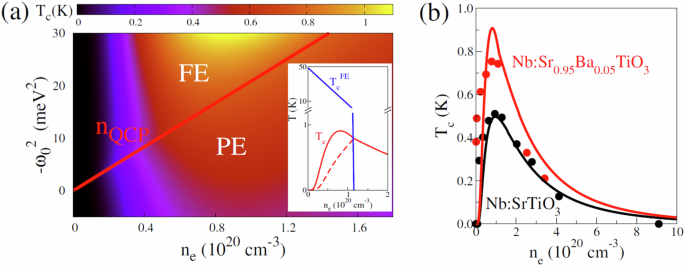
where the parameters take the values Γ ≈ 20.24 meV and β ≈ 0.09. This relationship is also illustrated in Fig. 3, which shows the coupling constant, gTO, as a function of carrier density, \({n}_{e}={k}_{F}^{3}/3{\pi }^{2}\).
Non-linear coupling
The QC Eliashberg theory predicts that the linear coupling favors the maximum Tc at the QCP, where it exhibits a cusp (except for small values of \({\omega }_{0}^{2}\)). However, this behavior contradicts experimental observations in Ba/Ca-doped STO, where the peak of the dome lies within the ordered phase28. Therefore, linear coupling alone cannot fully account for SC in Ba/Ca-doped STO. In this section, we explore beyond the linear order, i.e., the coupling to a pair of TO modes, which introduces a correction to the linear coupling, thereby enhancing the same.
The relative contribution of the linear and nonlinear coupling to pairing
To assess the relative contribution of the linear and nonlinear coupling to driving superconductivity, we evaluate here the pairing fluctuation associated with the two-phonon mechanism and compare it with the same arising from the linear coupling near the peak of the SC dome.
The vertex diagram for the quadratic coupling is shown in Fig. 9. The gap equation at the QCP assumes the form
$$\begin{array}{lll}\phi ({k}_{0})=\displaystyle\frac{{\lambda }^{{\prime} }{v}_{F}}{\pi }\displaystyle\int\,d{q}_{0}\displaystyle\int\,{d}^{3}q\,G(k+q)G(-k-q)\phi ({k}_{0}+{q}_{0})\displaystyle\frac{1}{{(2\pi )}^{4}{k}_{a}}\displaystyle\int\,d{q}_{0}^{{\prime} }\displaystyle\int\,{d}^{3}{q}^{{\prime} }\,D({q}^{{\prime} })D(q+{q}^{{\prime} })\\\\\qquad\quad ={\lambda }^{{\prime} }\int\,d{q}_{0}\displaystyle\frac{\phi ({k}_{0}+{q}_{0})}{| \tilde{\Sigma }({k}_{0}+{q}_{0})| }\displaystyle\int\,{d}^{2}q\,\displaystyle\frac{1}{{(2\pi )}^{4}{k}_{a}}\displaystyle\int\,d{q}_{0}^{{\prime} }\displaystyle\int\,{d}^{3}{q}^{{\prime} }\,D({q}^{{\prime} })D(q+{q}^{{\prime} })\\\\\qquad\quad ={\lambda }^{{\prime} }\displaystyle\int\,d{q}_{0}\displaystyle\frac{\phi ({k}_{0}+{q}_{0})}{| \tilde{\Sigma }({k}_{0}+{q}_{0})| }{d}_{NL}({q}_{0})\,.\end{array}$$
(49)
Here, we denote the quadratic coupling constant as \({\lambda }^{{\prime} }\), without delving into additional details in this section. For the detailed discussion of the coupling constant, please see the “Result” section (where we demonstrate \({\lambda }^{{\prime} }={\lambda }_{NL}{\langle {\boldsymbol{\eta }}\rangle }^{2}\)). The momentum integration in Eq. (49) is factorized as d3q → (1/vF)d2q∥dqϵ, where q∥ is parallel to the Fermi surface and qϵ is along the energy axis. We also drop the index (∥) in q∥, denoting it as q. Furthermore, the momenta are rescaled as q/ka → q and \({{\boldsymbol{q}}}^{{\prime} }/{k}_{a}\to {{\boldsymbol{q}}}^{{\prime} }\). In the last step of Eq. (49), we define a frequency-dependent kernel, dNL(q0), which is given by
$${d}_{NL}({q}_{0})=\frac{1}{{(2\pi )}^{4}{k}_{a}}\int\,d{q}_{0}^{{\prime} }\int\,{d}^{2}q\int\,{d}^{3}{q}^{{\prime} }\,D({q}^{{\prime} })D(q+{q}^{{\prime} })\,.$$
(50)
Here, the bosonic propagators, \(D({q}^{{\prime} })\) and \(D(q+{q}^{{\prime} })\), have a contribution from the Landau damped polarization bubble (\(\delta \Pi ({q}^{{\prime} })\) and \(\delta \Pi (q+{q}^{{\prime} })\), respectively).

The diagrammatic representation of the pairing vertex for nonlinear coupling. Two wavy lines represent boson propagators, and two solid lines represent fermion propagators.
To estimate the relative strength of pairing fluctuation from linear and quadratic couplings, we calculate the magnitude of the function dNL(q0) at the top of the dome and compare it with the bosonic function, d(q0), associated with the linear coupling. The magnitude of dNL(q0) is then given by
$$\begin{array}{lll}{d}_{NL}({q}_{0})&=&\displaystyle\frac{1}{{(2\pi )}^{4}{k}_{a}{v}_{F}}\displaystyle\int\,d{q}_{0}^{{\prime} }\displaystyle\int\,{d}^{2}{q}^{{\prime} }\displaystyle\int\,{d}^{2}q\mathop{\displaystyle\int}\nolimits_{-\infty }^{\infty }d{q}_{\epsilon }^{{\prime} }\\ &&\left(\frac{1}{| {{\boldsymbol{q}}}^{{\prime} }{| }^{2}+{{q}_{\epsilon }^{{\prime} }}^{2}+{\left(\frac{{q}_{0}^{{\prime} }\zeta }{c}\right)}^{2}+\delta \Pi ({q}^{{\prime} })}\right)\left(\frac{1}{| {\boldsymbol{q}}{| }^{2}+{{q}_{\epsilon }^{{\prime} }}^{2}+{\left(\frac{({q}_{0}+{q}_{0}^{{\prime} })\zeta }{c}\right)}^{2}+\delta \Pi (q+{q}^{{\prime} })}\right)\\ &=&\frac{\pi }{{(2\pi )}^{4}{k}_{a}{v}_{F}}\displaystyle\int\,d{q}_{0}^{{\prime} }\displaystyle\int\,{d}^{2}{q}^{{\prime} }\frac{\ln \left(\frac{\sqrt{| {{\boldsymbol{q}}}^{{\prime} }{| }^{2}+{\left(\frac{{q}_{0}^{{\prime} }\zeta }{c}\right)}^{2}+\delta \Pi ({q}^{{\prime} })}+\sqrt{{\left(\frac{({q}_{0}+{q}_{0}^{{\prime} })\zeta }{c}\right)}^{2}+\delta \Pi (q+{q}^{{\prime} })+{\left(\frac{\Lambda }{{k}_{a}}\right)}^{2}}}{\sqrt{| {{\boldsymbol{q}}}^{{\prime} }{| }^{2}+{\left(\frac{{q}_{0}^{{\prime} }\zeta }{c}\right)}^{2}+\delta \Pi ({q}^{{\prime} })}+\sqrt{{\left(\frac{({q}_{0}+{q}_{0}^{{\prime} })\zeta }{c}\right)}^{2}+\delta \Pi (q+{q}^{{\prime} })}}\right)}{\sqrt{| {{\boldsymbol{q}}}^{{\prime} }{| }^{2}+{\left(\frac{{q}_{0}^{{\prime} }\zeta }{c}\right)}^{2}+\delta \Pi ({q}^{{\prime} })}}\\ &=&\frac{\pi }{{(2\pi )}^{4}{k}_{a}{v}_{F}}\displaystyle\int\,d{q}_{0}^{{\prime} }F\left({\left(\frac{({q}_{0}+{q}_{0}^{{\prime} })\zeta }{c}\right)}^{2}+\delta \Pi (q+{q}^{{\prime} }),{\left(\frac{{q}_{0}^{{\prime} }\zeta }{c}\right)}^{2}+\delta \Pi ({q}^{{\prime} }),\frac{\Lambda }{{k}_{a}}\right)\,.\end{array}$$
(51)
Here, the UV cutoff for the integration over momentum is the Brillouin zone boundary Λ = π/a. The component \({q}_{\epsilon }^{{\prime} }\) is along the energy axis. We have also defined ζ = kB/ℏka. The function F(x, y, z) has the form
$$\begin{array}{lll}F(x,y,z)=\left(\sqrt{x}-\sqrt{x+{z}^{2}}\right)\ln \left(\sqrt{x}+\sqrt{y}\right)-\left(\sqrt{y}+\sqrt{x+{z}^{2}}\right)\ln \left(\frac{\sqrt{y}+\sqrt{x+{z}^{2}}}{\sqrt{x}+\sqrt{y}}\right)\\\qquad\qquad +\left(\sqrt{x+{z}^{2}}-\sqrt{x}\right)\ln \left(\sqrt{x}+\sqrt{y+{z}^{2}}\right)+\left(\sqrt{x+{z}^{2}}+\sqrt{y+{z}^{2}}\right)\ln \left(\frac{\sqrt{x+{z}^{2}}+\sqrt{y+{z}^{2}}}{\sqrt{x}+\sqrt{y+{z}^{2}}}\right)\,.\end{array}$$
(52)
At low temperatures, the first two arguments to F in Eq. (51) are always much smaller than the third, and we can approximate it as,
$$F(x,y,z)\approx 2\ln (2)z=\,\text{const}\,.$$
(53)
Near the top of the SC dome (at ne = 1 × 1020 cm−3), the Landau damped polarization bubble takes the value \(\delta \Pi =(\pi \bar{g}{\nu }_{F}/2)(c/{v}_{F})\approx 0.15\). The Fermi energy at this density is EF = 18.5 meV, and \(1/{v}_{F}{k}_{a}=2{\nu }_{F}{\pi }^{2}/{({k}_{F}a)}^{2}\) with νF = 0.24 eV−1. We consider q0 = 2πTc with Tc ≈ 1 K near the top of the dome. The lower limit of the integration in Eq. (51) is set to 2πTc and the upper limit is the Fermi level, EF/kB. We perform the integration numerically, which yields dNL = 4.9 × 10⁻³.
Now, let’s focus again on the kernel, d(q0), associated with the linear coupling (see Eq. (31)). It can be rewritten as
$$d({q}_{0})=\mathop{\int}\nolimits_{0}^{\Lambda /{k}_{a}}{d}^{2}q\left(\frac{1}{| {\boldsymbol{q}}{| }^{2}+{\left(\frac{{q}_{0}\zeta }{c}\right)}^{2}+\delta \Pi (q)}\right)=\frac{1}{2}\ln \left(1+\frac{{\left(\frac{\Lambda }{{k}_{a}}\right)}^{2}}{{\left(\frac{{q}_{0}\zeta }{c}\right)}^{2}+\delta \Pi (q)}\right)\,.$$
(54)
At the top of the dome, Eq. (54) yields a value d = 2.1. Thus, the ratio of the bosonic kernels associated with the quadratic and linear couplings at the top of the dome is obtained as dNL/d ~ 2.3 × 10⁻³, which reveals the dominance of the linear coupling over the nonlinear coupling.
The role of Landau damping in the nonlinear coupling at the high-density limit
In the “Results” section, we discussed that in the moderate to high density regime, the linear coupling plays a dominant role in driving superconductivity in Ba/Ca-doped STO. Once the FE moment develops a finite expectation value, an additional correction from nonlinear coupling emerges, capturing finer features near the QCP. However, the non-linear coupling can also contribute to pairing from the fluctuations around the mean (the so-called two-phonon coupling or Ngai mechanism). Van der Marel et al.53 were the first to apply the two-phonon mechanism to the soft FE mode in STO. Through optical conductivity measurements, they estimated the coupling and concluded that it is a relevant mechanism. Kiselov and Feigelman54 further applied this two-phonon coupling model to the extremely low-density regime (ne 18 cm−3), where only one electronic band is occupied. In their treatment of the low-density limit, they made two key approximations: the renormalization of the phonon frequency ωT due to carrier concentration was neglected, and the effective interaction was assumed to be static. Despite these simplifications, the results were in good agreement with the measured critical temperature Tc2. Volkov et al.55 studied the two-phonon coupling close to the quantum-critical point to describe superconductivity in doped STO. However, the results are best justified at the extreme low-density limit, where the Fermi surface is sufficiently small to satisfy the antiadiabetic limit (Fermi energy, EF ωT), in accord with ref. 54.
In this section, we estimate how important the Landau damping correction is in the two-phonon process near the top of the dome. We analyze dNL(q0) (defined in Eq. (50)). We perform the integral in a slightly more transparent but approximate fashion by integrating over momenta independently. After the integration over momenta, q and \({q}^{{\prime} }\), up to the Brillouin zone boundary Λ = π/a, the kernel takes the form
$$\begin{array}{lll}{d}_{NL}({q}_{0})\approx \frac{1}{{(2\pi )}^{4}{k}_{a}{v}_{F}}\int\,d{q}_{0}^{{\prime} }\int\,d{q}_{\epsilon }^{{\prime} }\int\,{d}^{2}{q}^{{\prime} }\left(\frac{1}{| {{\boldsymbol{q}}}^{{\prime} }{| }^{2}+{{q}_{\epsilon }^{{\prime} }}^{2}+{\left(\frac{{q}_{0}^{{\prime} }\zeta }{c}\right)}^{2}+\delta \Pi ({q}^{{\prime} })}\right)\\\\\qquad\qquad\quad \times \int\,{d}^{2}q\left(\frac{1}{| {\boldsymbol{q}}{| }^{2}+{{q}_{\epsilon }^{{\prime} }}^{2}+{\left(\frac{({q}_{0}+{q}_{0}^{{\prime} })\zeta }{c}\right)}^{2}+\delta \Pi (q+{q}^{{\prime} })}\right)\\\\\qquad\quad\,\,\,\,\,\, =\frac{1}{{(2\pi )}^{4}{k}_{a}{v}_{F}}\int\,d{q}_{0}^{{\prime} }\int\,d{q}_{\epsilon }^{{\prime} }\ln \left[\frac{\Lambda /{k}_{a}}{{\left({{q}_{\epsilon }^{{\prime} }}^{2}+{\left(\frac{{q}_{0}^{{\prime} }\zeta }{c}\right)}^{2}+\delta \Pi ({q}^{{\prime} })\right)}^{1/2}}\right]\\\\\qquad\qquad\quad \times \ln \left[\frac{\Lambda /{k}_{a}}{{\left({{q}_{\epsilon }^{{\prime} }}^{2}+{\left(\frac{({q}_{0}+{q}_{0}^{{\prime} })\zeta }{c}\right)}^{2}+\delta \Pi (q+{q}^{{\prime} })\right)}^{1/2}}\right]\,.\end{array}$$
(55)
Here, we have shifted the integration variable \({\boldsymbol{q}}\to {\boldsymbol{q}}-{{\boldsymbol{q}}}^{{\prime} }\). The UV momentum cutoff is the Brillouin zone boundary Λ = π/a. The Landau damped polarization bubble (\(\delta \Pi ({q}^{{\prime} })\) and \(\delta \Pi (q+{q}^{{\prime} })\)) sets an IR cutoff scale for the momentum integration. The results of ref. 55 are reproduced in the limit vF ≪ c, and when neglecting the Landau damping. Indeed, in this case, Eq. (55) simplifies to \({d}_{NL} \sim {k}_{F}^{2}\ln \left(\Lambda /c{k}_{F}\right)\).
To extend the solution of Tc to the higher densities, it is essential to estimate the typical magnitude of δΠ and determine when it is a relevant cutoff. In the space of frequency and momentum, it dominates the bosonic function INL when
$${\left(\frac{{q}_{0}^{{\prime} }}{c}\right)}^{2}
(56)
We recall that \(\gamma =\pi \bar{g}{\nu }_{F}/2{v}_{F}\) with \(\bar{g}=4{g}_{TO}^{2}{({k}_{F}a)}^{2}{D}_{0}\) (see Eq. (8), Eq. (13), and Eq. (27)). Using these expressions with the assumption that \(| {q}_{0}^{{\prime} }”https://www.nature.com/” {{\boldsymbol{q}}}^{{\prime} } \sim c\), Eq. (56) assumes the form
$${q}_{0}^{{\prime} }
(57)
and δΠ takes the value
$$\frac{\sqrt{\delta \Pi }}{{k}_{F}} \sim \frac{{g}_{TO}\sqrt{{D}_{0}}}{\sqrt{\pi {E}_{F}}}{\left({k}_{F}a\right)}^{3/2}\,.$$
(58)
We use Eq. (58) to estimate δΠ near the peak of the dome (at ne = 1 × 1020 cm−3), where gTO ≈ 45.3 meV and kFa ≈ 0.56, which leads to \(\sqrt{\delta \Pi }/{k}_{F} \sim 2.5\). Therefore, we conclude that the Landau damping term δΠ can not be neglected in FE-doped STO for densities near the peak of the dome or above it.
Gap equation for the generalized Rashba coupling
In the FE ordered phase, the nonlinear coupling provides a correction to the linear coupling. We now turn our attention to the generalized Rashba coupling, which is described by the Lagrangian
$${L}_{Rashba}\approx {\left(\frac{a}{L}\right)}^{3}\sum _{{\boldsymbol{k}},{\boldsymbol{q}}}{\psi }_{\alpha }^{\dagger }\left({\boldsymbol{k}}+\frac{{\boldsymbol{q}}}{2}\right){\boldsymbol{\eta }}({\boldsymbol{q}})\cdot \left(\hat{k}\times {{\boldsymbol{\sigma }}}_{\alpha \gamma }\right)\left[g\,{\delta }_{\gamma \beta }+{g}_{NL}\,\langle {\boldsymbol{\eta }}\rangle \cdot \left(\hat{k}\times {{\boldsymbol{\sigma }}}_{\gamma \beta }\right)\right]{\psi }_{\beta }\left({\boldsymbol{k}}-\frac{{\boldsymbol{q}}}{2}\right)\,.$$
(59)
Here, the transverse displacement vector is denoted by η. The first term represents the linear Rashba coupling, where the coupling constant is denoted by g. The second term with a coupling constant, gNL captures the nonlinear correction. The equation for the pairing vertex associated with this coupling can be written as
$$\begin{array}{lll}{\Phi }_{\alpha \beta }(k)=\bar{g}\displaystyle\frac{T}{{k}_{a}^{3}}\sum _{{p}_{0}}\displaystyle\int\displaystyle\frac{{d}^{3}p}{{(2\pi )}^{3}}G(p)G(-p)D(p-k){{\boldsymbol{\gamma }}}^{\nu \alpha }(-\hat{k}){\Phi }_{\nu \mu }(k)\cdot \hat{P}(\hat{q})\cdot {{\boldsymbol{\gamma }}}^{\mu \beta }(\hat{k})\\\\\qquad\quad +4{\bar{g}}_{NL}{\langle {\boldsymbol{\eta }}\rangle }^{2}\displaystyle\frac{T}{{k}_{a}^{3}}\sum _{{p}_{0}}\displaystyle\int\displaystyle\frac{{d}^{3}p}{{(2\pi )}^{3}}G(p)G(-p)D(p-k)\\\\\qquad\quad \times {{\boldsymbol{\gamma }}}^{\tau \alpha }(-\hat{k}){{\boldsymbol{\gamma }}}^{\gamma \tau }(-\hat{k})\cdot \hat{P}(\hat{q}){\Phi }_{\gamma \mu }(k)\cdot \hat{P}(\hat{q})\cdot {{\boldsymbol{\gamma }}}^{\mu \nu }(\hat{k}){{\boldsymbol{\gamma }}}^{\nu \beta }(\hat{k})\,.\end{array}$$
(60)
Here, we have defined the coupling constants as \(\bar{g}={g}^{2}{D}_{0}\), and \({\bar{g}}_{NL}={g}_{NL}^{2}{D}_{0}\) for linear and nonlinear coupling, respectively. We consider the attractive singlet channel. We have already discussed the spin summation and projection on the transverse sector for the linear coupling corresponding to the first term in Eq. (60) (see Eq. (34)). We proceed with the second term in Eq. (60) (the quadratic coupling) in a similar fashion, which leads to
$$\begin{array}{lll}\\\quad4{\langle {\boldsymbol{\eta }}\rangle }^{2}{\left(-\hat{k}\times {\boldsymbol{\sigma }}\right)}_{\tau \alpha }{\left(-\hat{k}\times {\boldsymbol{\sigma }}\right)}_{\gamma \tau }\cdot \hat{P}(\hat{q}){\Phi }_{\gamma \mu }({p}_{0},{\boldsymbol{k}})\cdot \hat{P}(\hat{q})\cdot {\left(\hat{k}\times {\boldsymbol{\sigma }}\right)}_{\mu \nu }{\left(\hat{k}\times {\boldsymbol{\sigma }}\right)}_{\nu \beta }\\ =4{\langle {\boldsymbol{\eta }}\rangle }^{2}i{\sigma }_{y}\left({\sigma }_{t}{\sigma }_{t}+{\sigma }_{u}{\sigma }_{u}\right)\phi ({p}_{0})\left(\cos \phi {\sigma }_{t}-\sin \phi {\sigma }_{u}\right)\left(\cos \phi {\sigma }_{t}-\sin \phi {\sigma }_{u}\right)\\ =8{\langle {\boldsymbol{\eta }}\rangle }^{2}i{\sigma }_{y}\phi ({p}_{0})\,.\end{array}$$
(61)
Eq. (60) can now be simplified as
$$\begin{array}{lll}\phi ({k}_{0})=\frac{\bar{g}+8{\bar{g}}_{NL}{\langle {\boldsymbol{\eta }}\rangle }^{2}}{{k}_{a}^{3}}T\mathop{\sum}\limits _{{p}_{0}}\int\frac{{d}^{3}p}{{(2\pi )}^{3}}G(p)\phi ({p}_{0})G(-p)D(p-k)\\\\\qquad\quad =(\lambda +{\lambda }_{NL}{\langle {\boldsymbol{\eta }}\rangle }^{2})T\mathop{\sum}\limits _{{p}_{0}}\frac{d({p}_{0}-{k}_{0})\phi ({p}_{0})}{| {p}_{0}+\Sigma ({p}_{0})| }\,.\end{array}$$
(62)
Here, the effective coupling constant for the linear and nonlinear couplings is represented by \(\lambda =\bar{g}{\nu }_{F}{k}_{a}^{2}/4{k}_{F}^{2}\) and \({\lambda }_{NL}{\langle {\boldsymbol{\eta }}\rangle }^{2}=2{\bar{g}}_{NL}{\nu }_{F}{k}_{a}^{2}{\langle {\boldsymbol{\eta }}\rangle }^{2}/{k}_{F}^{2}\), respectively. We exclude the diverging contribution of d(p0−k0) at k0 = p0 and define a new gap function \(\Delta ({k}_{0})={k}_{0}\,\phi ({k}_{0})/\tilde{\Sigma }({k}_{0})\), which results in
$$\Delta ({k}_{0})=\frac{(\lambda +{\lambda }_{NL}{\langle {\boldsymbol{\eta }}\rangle }^{2})T{\sum }_{{p}_{0}\ne {k}_{0}}\frac{\Delta ({p}_{0})}{{p}_{0}}\left[d({p}_{0}-{k}_{0})+d({p}_{0}+{k}_{0})\right]}{1+(\lambda +{\lambda }_{NL}{\langle {\boldsymbol{\eta }}\rangle }^{2})T\frac{1}{{k}_{0}}{\sum }_{{q}_{0}\ne {k}_{0}}\left[d({q}_{0}-{k}_{0})-d({q}_{0}+{k}_{0})\right]}\,.$$
(63)
We solve this equation to calculate Tc, as shown in the Results.
Additional information on the numerical computation and the theoretical resultsThe phase diagram
The calculated Tc, obtained from Eq. (47) (associated with the linear coupling) and Eq. (63) (associated with the enhanced linear coupling from the nonlinear correction), is shown in Fig. 10a, b, respectively. In both panels, Tc is plotted as a function of \(-{\omega }_{0}^{2}\) and carrier density, ne, with ne shown on a logarithmic scale. The results in panel a and b are identical to those in Figs. 4b and 5b, respectively, where carrier density, ne, is presented on a linear scale.
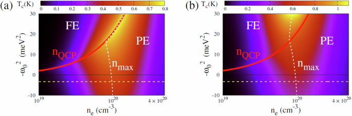
Tc is shown as a function of carrier density ne (plotted on a logarithmic scale) and frequency \({\omega }_{0}^{2}\) (plotted on a linear scale). a Corresponds to the linear coupling, and b corresponds to the effective enhancement of the linear coupling from nonlinear contribution (b = 49 meV2). The yellow dashed line in both panels marks STO without FE doping (\({\omega }_{0}^{2}=3.3\) meV2). The red solid line in both panels denotes nQCP and the white dashed line indicates the peak of the SC dome, \({n}_{\max }\).
Truncated linear coupling
In our Results, we demonstrated that the QC Eliashberg theory with linear coupling produces a peak in the SC dome at the QCP, resulting in a cusp at \({n}_{\max }={n}_{QCP}\), given that \({\omega }_{0}^{2}\) (λ, remains density independent. Here, we show that the maximum Tc can shift away from the QCP into the ordered phase when the coupling is truncated at large density. We incorporate a density cutoff in the linear coupling,gTO, for density \({n}_{e} > {n}_{e}^{m}\) \({n}_{e}^{m}\) is the density where gTO is maximum) with a “Fermi function”. The modified bare coupling \({g}_{TO}^{c}\) is given by
$${g}_{TO}^{c}={g}_{TO}\left[\frac{1}{1+\exp \left(\frac{{n}_{e}-\alpha \,{n}_{e}^{m}}{\beta \,1{0}^{20}}\right)}\right]\,.$$
(64)
The purpose of using the “Fermi function” is to truncate gTO in the high-density regime, while preserving its behavior in the low-density regime. The parameters α and β govern the range of these two regimes, along with the decay rate at large density. The modified couplings, \({g}_{TO}^{c}\) and \({\lambda }^{c}={({g}_{TO}^{c})}^{2}{D}_{0}{\nu }_{F}\) with α = 4 and β = 0.2 are shown in Fig. 11a by the dashed lines. These parameter values indicate a strong decay chosen to enable a prominent comparison of Tc with the previous results. The truncated coupling, λc, increases with density in the low-density regime and decreases in the high-density regime. In the intermediate regime, around ne = 0.9 × 1020 cm−3, λc exhibits a weak density dependence, forming a rounded top. This behavior arises as an artifact of the “Fermi function”.
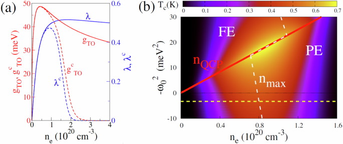
a The red lines represent the bare electron-phonon coupling (left y axis) and the blue lines denote the effective coupling constant (right y axis) as a function of carrier density ne. The solid lines represent the linear coupling gTO15 (see Eq. (48)) and \(\lambda ={g}_{TO}^{2}{D}_{0}{\nu }_{F}\) and the dashed lines denote the truncated couplings \({g}_{TO}^{c}\) (see Eq. (64)) and \({\lambda }^{c}={({g}_{TO}^{c})}^{2}{D}_{0}{\nu }_{F}\) with α = 4 and β = 0.2. b The color map represents Tc as a function of ne and \(-{\omega }_{0}^{2}\) along x axis and y axis, respectively. The results correspond to the truncated coupling \({g}_{TO}^{c}\) with α = 4 and β = 0.2. Additionally, \({g}_{TO}^{c}\) is rescaled (\({g}_{TO}^{c}\to {g}_{TO}^{c}/1.1\)) such that the maximum Tc for \({\omega }_{O}^{2}=3.3\) agrees with the experimentally measured value of the same for STO without FE doping. The yellow dashed line marks STO without FE doping (\({\omega }_{0}^{2}=3.3\) meV2). The red solid line denotes nQCP and the white dashed line shows the peak position of the SC dome, \({n}_{\max }\).
We solve the gap equation in Eq. (47) by replacing λ with the truncated effective coupling λc. The resulting Tc is shown by the color map in Fig. 11b as a function of carrier density, ne, and \({\omega }_{0}^{2}\). The position of the dome peak, \({n}_{\max }\), is indicated by the white dashed line, and the red solid line represents nQCP. The figure shows that the dome peak shifts to the lower density as \({\omega }_{0}^{2}\) decreases (when \({\omega }_{0}^{2}\) is small, whether positive or negative). At a certain value of \({\omega }_{0}^{2}\) (\({n}_{\max }\) reaches the QCP. The dome peak coincides with the QCP for a small range of \({\omega }_{0}^{2}\) (λc in the intermediate density regime. As \({\omega }_{0}^{2}\) decreases further, the dome peak shifts into the ordered state. However, λc at nQCP is significantly suppressed in this regime, resulting in reduced values of Tc.
Superconductivity in Ca-doped, Zr-doped, and 18O isotope-substituted STO
The results presented in the previous sections, correspond to Ba-doped STO. Here we focus on three additional systems, i.e., \({{\rm{Sr}}}_{1-z}{{\rm{Ca}}}_{z}{{\rm{Ti}}}_{1-{z}^{{\prime} }}{{\rm{Nb}}}_{{z}^{{\prime} }}{{\rm{O}}}_{3}\), SrTi(18\({{{\rm{O}}}_{y}^{16}{{\rm{O}}}_{1-y}\left.\!\right)}_{3-\delta }\)5 and SrTi1−xZrxO3−δ82. The SC phase diagram for Ca-doped STO is shown in Fig. 12a. Panel (b) of the same figure depicts excellent agreement between the calculated Tc and the experimental data at Ca content z = 0.015 (\({\omega }_{0}^{2}=-6.2\) meV2, also marked by yellow dashed line in panel (a)), as reported in ref. 28. The FE order, induced by 18O substitution, is confined to extremely low carrier densities, and the SC dome resides in the PE state5 where the nonlinear coupling correction is negligible. Consequently, the SC phase diagram in Fig. 13a, derived using only linear coupling, shows excellent agreement with experimental results.
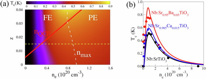
a Tc, calculated at b = 49 meV2, as a function of ne and Ca content z in \({{\rm{Sr}}}_{1-z}{{\rm{Ca}}}_{z}{{\rm{Ti}}}_{1-{z}^{{\prime} }}{{\rm{Nb}}}_{{z}^{{\prime} }}{{\rm{O}}}_{3}\) along x axis and y axis, respectively. The yellow dashed horizontal line marks Sr0.985Ca0.015TiO328 (\({\omega }_{0}^{2}=-6.2\,{{\rm{meV}}}^{2}\)). The red solid line denotes nQCP and the white dashed line shows the peak position of the SC dome, \({n}_{e}={n}_{\max }\). b Comparison between the theoretical Tc (solid lines) and experimental Tc (filled circles) for FE undoped, Ba-doped, and Ca-doped STO (from ref. 28).
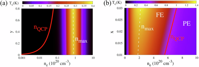
Tc is shown as a function of carrier density ne and doping content (18O content y in a and Ba content x in b). The corresponding nQCP (the red solid lines in both panels) as a function of doping content is extracted from refs. 5 and. 82, respectively. Tc in a is obtained by solving the gap equation for linear coupling (Eq. (47)) in a, while the result in b is obtained from the gap equation Eq. 63 at b = 100 meV2. The white dashed line in both panels indicates the peak of the SC dome, \({n}_{\max }\).
On the contrary, doping with Zr results in a substantially large nQCP, and superconductivity emerges deep in the FE state. Increasing the doping concentration elevates nQCP, driving the SC regime further away from QC, and consequently, suppressing Tc rather than enhancing it82. In this specific case, our simplified model, which is only quartic in the order parameter, cannot capture the suppression deep in the ordered state. The reason is that the displacement grows in the ordered state as 〈η〉2 = ∣r∣/b, neglecting its saturation deep in the ordered state. While this assumption is valid near the QCP, it tends to enhance Tc by overestimating the nonlinear coupling correction in the deep FE state, thereby limiting a quantitative prediction of Tc for Zr-doped STO. This is evident in the phase diagram in 13b, calculated using the nonlinear coupling correction for b = 100 meV2. It demonstrates that while the variation of \({n}_{\max }\) with Zr content x agrees with experimental observations, Tc is enhanced with x. Reducing the nonlinear correction further (b = 400 meV2) results in suppression of Tc.
Rescaled frequency
We have presented the gap equations for the linear coupling and the enhanced linear coupling, incorporating the nonlinear correction, in Eq. (47) and Eq. (63), respectively. In both expressions, the upper cutoff of the summations over fermionic frequency p0 = (2m + 1)πT is fixed at the Fermi level fc = EF/kB. The frequency index m is an integer. For a fixed maximum frequency index M we redefine the energy scale of frequencies with index m > mrg, while keeping the regular energy scale for index m mrg88. The rescaled frequencies can be presented as
$$\begin{array}{lll}{p}_{0}=(2m+1)\pi T,\qquad \qquad \qquad \qquad \quad m
(65)
These expressions suggest that the modified frequency indices for m > mrg are given by meff = m + eam−b. The rescaled frequency indices are separated from each other by
$$\begin{array}{lll}df(m)=1\,,\qquad \qquad \qquad \qquad \qquad \quad m
(66)
The parameters, a and b, are chosen so that the deviation from the regular frequency scale at m = mrg is tiny (s). This deviation gradually increases with higher indices, eventually reaching the desired upper cutoff frequency, fc, at m = M. Additionally, the upper limit fc can be defined in terms of the regular frequency indices as fc = (2k + 1)πT. Thus, Eq. (65) leads to
$$\begin{array}{l}{m}_{rg}+{e}^{a{m}_{rg}-b}={m}_{rg}+s\,,\\ a{m}_{rg}-b=\ln s\,.\end{array}$$
(67)
$$\begin{array}{l}M+{e}^{aM-b}=k\,,\\ aM-b=\ln (k-M)\,.\end{array}$$
(68)
Now, from Eq. (67), and (68), we obtain
$$\begin{array}{lll}a=\displaystyle\frac{\ln (k-M)-\ln s}{M-{m}_{rg}}\,,\\ b=\displaystyle\frac{{m}_{rg}\ln (k-M)-M\ln s}{M-{m}_{rg}}\,.\end{array}$$
(69)
In Fig. 14, we plot meff as a function of m with three different values of M (M = 20, 50, and 100). The parameters used are mrg = 10, frequency shift s = 0.1 from the regular frequency at m = mrg, and k = 1000. The figure demonstrates how the M frequency indices effectively span the entire energy range up to fc.
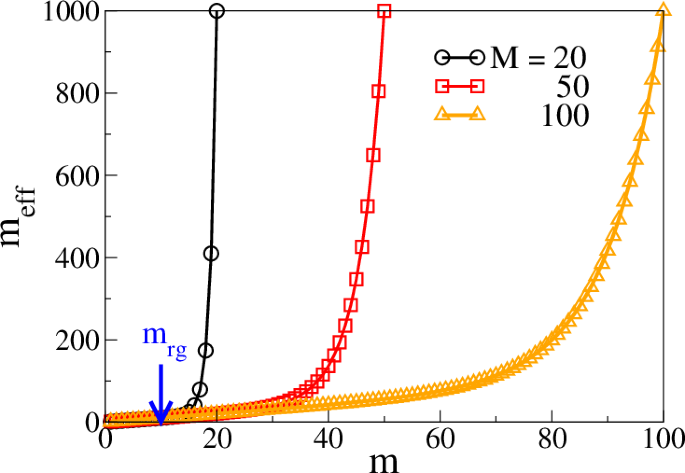
The new frequency index meff grows to k = 1000 at m = M. We choose three different values of M as M = 20, 50, 100. The highest index cutoff of the regular frequency scale in the rescaled frequency, mrg = 10, is marked by the arrow.
Finally, let’s assume that the indices for frequencies p0 and q0 in Eq. (47) and Eq. (63) are m and n, respectively. We use the rescaled frequencies in these expressions. Thus, Eq. (47) is modified as
$$\Delta ({k}_{0})=\frac{\lambda T{\sum }_{{p}_{0}\ne {k}_{0}}df(m)\frac{\Delta ({p}_{0})}{{p}_{0}}\left[d({p}_{0}-{k}_{0})+d({p}_{0}+{k}_{0})\right]}{1+\lambda T\frac{1}{{k}_{0}}{\sum }_{{q}_{0}\ne {k}_{0}}df(n)\left[d({q}_{0}-{k}_{0})-d({q}_{0}+{k}_{0})\right]}\,.$$
(70)
Similarly, Eq. (63) is modified as
$$\Delta ({k}_{0})=\frac{(\lambda +{\lambda }_{NL}{\langle {\boldsymbol{\eta }}\rangle }^{2})T{\sum }_{{p}_{0}\ne {k}_{0}}df(m)\frac{\Delta ({p}_{0})}{{p}_{0}}\left[d({p}_{0}-{k}_{0})+d({p}_{0}+{k}_{0})\right]}{1+(\lambda +{\lambda }_{NL}{\langle {\boldsymbol{\eta }}\rangle }^{2})T\frac{1}{{k}_{0}}{\sum }_{{q}_{0}\ne {k}_{0}}df(n)\left[d({q}_{0}-{k}_{0})-d({q}_{0}+{k}_{0})\right]}\,.$$
(71)