
In this study, we use a 2D distorted pores and throats network. As a base case, we consider the networks to be initially oil-wet with contact angles equal to 140o. The initial viscous ratio is equal to 10 (\(\:{\mu\:}_{water}\)= 1cP, \(\:{\mu\:}_{oil}\) = 10cP), and water is injected with an average frontal advance velocity V equal to 1 m/day. LS brine gradually shifts the contact angles from 140o to 95o, whilst polymer modifies water viscosity from 1cP to 10cP. Table 1 summarises the network properties and flow parameters used in the base case study.
Seed number
The 2D statistically generated networks used in this study sample pore radii from a predefined pore size distribution. A random seed is a parameter used by random number generators to ensure that whenever we sample a sequence of numbers from a random distribution, we always end up with the same sequence – this can be useful when wanting to compare different flooding sequences on an identical network. However, running a single simulation using a single seed cannot be considered a very reliable approach to quantify the effect of a particular flooding protocol and so we run multiple simulations for each scenario by using multiple seeds. In this study, every scenario has been carried out using 5 different networks that share the same average properties, but which differ on a local scale. The results are consequently presented as statistical distributions rather than single data points.
Model results
To explain some of the observations, we will make use of the Regime index, \(\:{R}^{index}\) which measures the dominant force during a flood: \(\:{R}^{index}>0\) implies viscous perturbation and \(\:{R}^{index} implies capillary dominance. Viscous dominance usually begins somewhere around \(\:{R}^{index}>1\) meaning that the viscous force is at least twice the capillary resistance. For \(\:0, there is a transition between capillary and viscous regimes. \(\:{R}^{index}\) is a useful indicator and is calculated at each timestep by the equations:
$$\:\stackrel{-}{{P}_{c}}=\frac{1}{n}\sum_{i=1}^{n}2\sigma\:\text{cos}\theta\:/{R}_{i}$$
(8)
$$\:{R}^{index}=(\varDelta\:P-{\stackrel{-}{P}}_{c})/{\stackrel{-}{P}}_{c}$$
(9)
where n is the current number of water filled elements, Ri is the radius of water filled element i, \(\:\sigma\:\) is the oil-water interfacial tension, \(\:\theta\:\) is the contact angle, \(\:\stackrel{-}{{P}_{c}}\) is the current mean capillary pressure in the network and \(\:\varDelta\:P\) is the current pressure gradient across the network.
LS Brine injection
We begin by comparing the first injection sequence where the following cases are considered (i) High salinity water is injected for 3PVs (ii) high salinity (HS) water is first injected to Sor and then replaced by LS brine till a total of 3PVs injected (iii) HS water is injected to an intermediate saturation and then replaced with LS brine for a total of 3PVs (iv) LS brine is injected in secondary mode for 3PVs.
For a mobility ratio of 10 and frontal advance velocity of 1 m/day and the base network data presented in Table 1, \(\:{\varvec{S}}_{\varvec{o}\varvec{r}}^{\varvec{H}\varvec{S}}\) is reached at approximately 0.65PVs injected and breakthrough of HS water occurs after 0.35PV.
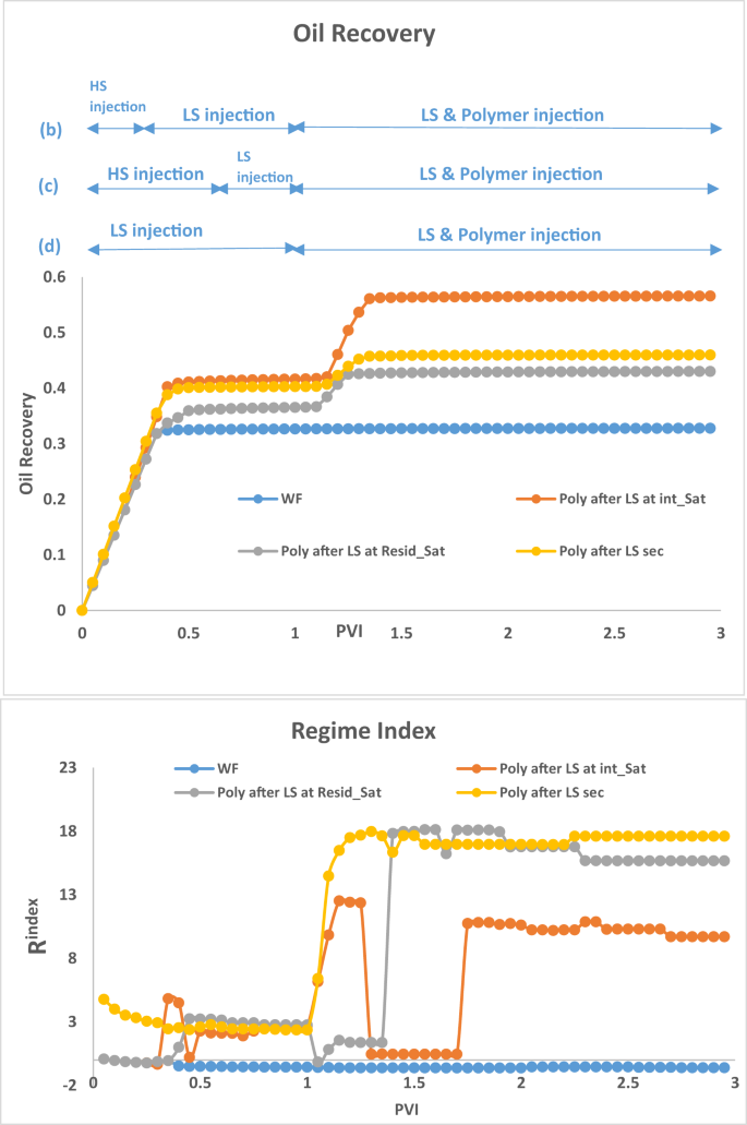
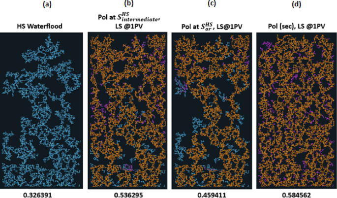
The results in Fig. 3, can be interpreted by examining the Rindex in Fig. 4. For the HS water waterflood (Fig. 3(a)), the displacement process is capillary dominated, giving rise to large clusters of bypassed oil due to capillary resistance and the pressure gradient being unable to displace extra oil. When LS brine is injected after 1PV of HS brine (Fig. 3(c)) (which is after residual oil saturation, \(\:{\varvec{S}}_{\varvec{o}\varvec{r}}^{\varvec{H}\varvec{S}}\), has been reached), the injected LS brine travels along existing HS pathways and is only able to displace some additional oil from its direct neighbours, with most of the flow being through established pathways.
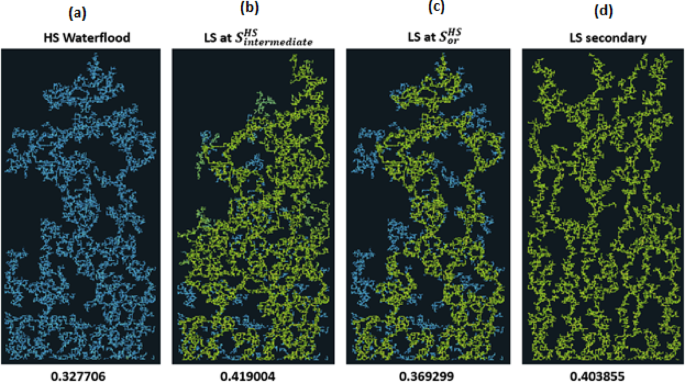
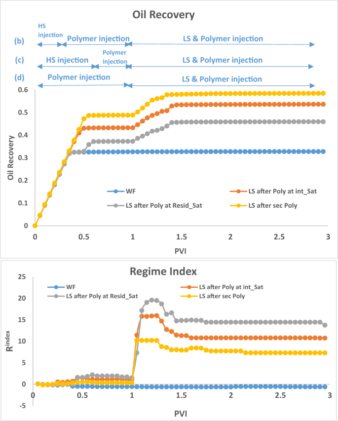
Water distribution after 3PVs injected, M = 1, v = 1 m/day. From Left to right: (a) HS water flood (b) HS water replaced with LS brine after several PVs before breakthrough of HS water (c) HS water replaced with LS brine after residual saturation of oil is reached (d) Secondary injection of LS brine.
The LS brine is still able to affect the capillary entry pressure of its directly connected oil-filled neighbours but is unable to greatly influence the pressure distribution, which is why the regime index is the same as that seen in the HS waterflood. This flood yields an additional 4% oil recovery. When LS brine is injected at an intermediate saturation (0.25PVs, Fig. 3(b)) we see a change in regime index starting from around 0.3PV and the subsequent shift to a viscous dominated displacement. Also, the displacement is more stable when LS brine is injected at an intermediate saturation before breakthrough. This limits the capillary fingering that would have developed without LS brine injection. The oil recovery plot shows that while the recovery for HS water plateaued at approximately 0.3PVI, the recovery from LS brine injection initiated at an intermediate HS saturation continued to rise with ~ 10% more oil being recovered until it plateaued at 0.45PVI. When LS brine is injected in secondary mode (Fig. 3(d)), the displacement is viscous dominated from the start of injection, and we observe a viscous fingering pattern in the displacement due to the change in contact angle (wettability). Although smaller pore sizes are now accessible to the displacing phase, this change in regime and the elongation of the water clusters leads to more bypassed oil and recovery is not optimised.

Oil recovery and Regime index plots after 3PVs injected for HS waterflood and LS brine injection for Sequence 1–3.
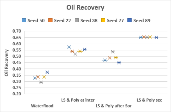
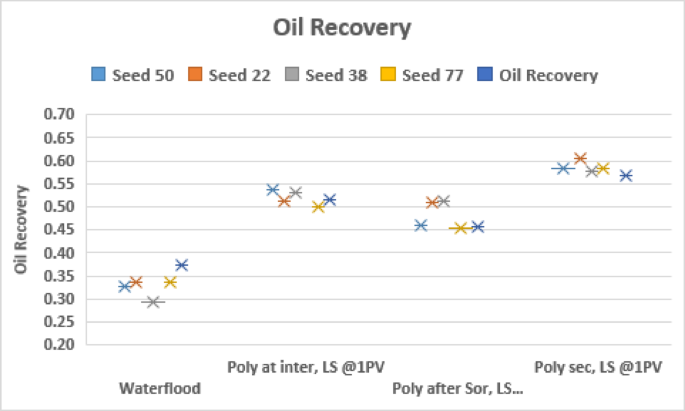
To confirm the observation of a more stable displacement pattern when LS brine is injected following an intermediate HS saturation before breakthrough, we repeat the simulation for 5 different networks represented by different seed numbers. This is shown in Fig. 5.
The results for the different network structures confirm that the benefit of LS brine injection is impacted by the timing of the injection: we see better performance when LS brine is injected in general but maximising the recovery potential might require injecting LS brine before breakthrough of HS brine, rather than injecting LS brine from the start of the water flood.
This can be explained by the observation that, in secondary injection of LS, the capillary forces are altered at the start of the waterflood and the flow regime is unstable viscous fingering, oil is bypassed in the process and flow takes the shortest paths to the outlet. When LS brine is injected at an intermediate HS saturation, the flow is initially capillary dominated and the brine is better connected in the transverse direction: the subsequent introduction of LS brine to alter the wettability and reduce capillary resistance means the LS brine has access to more areas of the network and can advance in a more stable way, displacing more oil in the process.
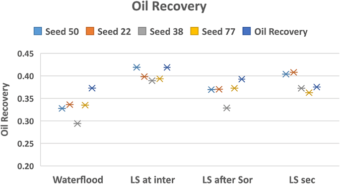
Oil recovery for injection sequences 1–3 and HS waterflood after 3PVs injected for M = 10 across 5 different capillary networks, v = 1 m/day.
LS Brine and polymer simultaneously
If we consider the previous sequences, but now with polymer injected simultaneously with LS brine after \(\:{\varvec{S}}_{\varvec{o}\varvec{r}}^{\varvec{H}\varvec{S}}\), at \(\:{\varvec{S}}_{\varvec{i}\varvec{n}\varvec{t}\varvec{e}\varvec{r}\varvec{m}\varvec{e}\varvec{d}\varvec{i}\varvec{a}\varvec{t}\varvec{e}}^{\varvec{H}\varvec{S}}\) and with LS brine in secondary mode, the final distribution is shown in Fig. 6.
The simultaneous injection of LS brine and polymer in general gives a better recovery than LS brine injection on its own. For the case of LS brine and polymer injection after \(\:{\varvec{S}}_{\varvec{o}\varvec{r}}^{\varvec{H}\varvec{S}}\) the displacement follows the existing pathways established by the HS water flood for much of the injection but recovers some additional oil from the directly connected neighbours after the reduction in the capillary entry pressure (due to LS effect and the increased pressure gradient from the polymer injection). This yields an increase of 12% in comparison to the HS waterflood, and more than 7% in comparison with only LS brine injection at this point.
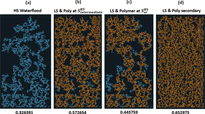
Water distribution after 3PVs injected for M = 10, v = 1 m/day. From Left to right: (a) HS water flood for 3PVs (b) HS water is injected to an intermediate saturation, then replaced with LS brine and polymer injected simultaneously (c) HS water is injected to Sor then replaced with LS brine and polymer simultaneously (d) LS brine and polymer simultaneously injected in secondary mode.
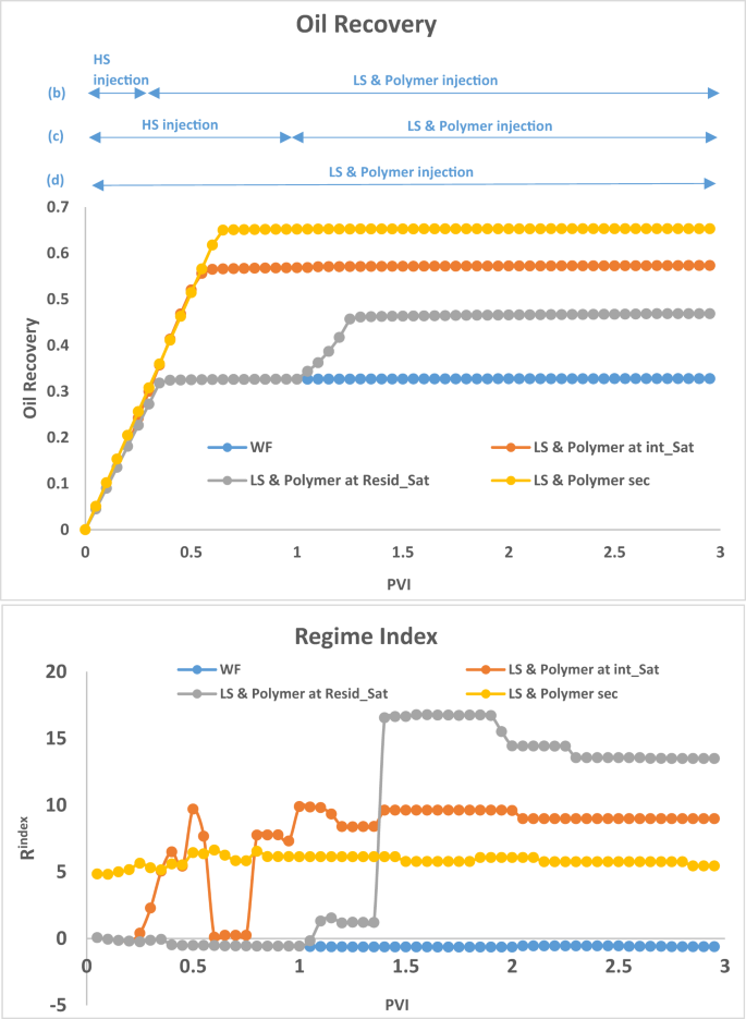
Oil recovery and Regime index plots for HS waterflood and injection sequences 4–6 after 3PVs injected M = 10, v = 1 m/day.
For LS brine and polymer injection at \(\:{\varvec{S}}_{\varvec{i}\varvec{n}\varvec{t}\varvec{e}\varvec{r}\varvec{m}\varvec{e}\varvec{d}\varvec{i}\varvec{a}\varvec{t}\varvec{e}}^{\varvec{H}\varvec{S}}\) (Fig. 6(b)), although LS brine injection on its own was able to displace additional oil, with polymer, the injected fluid can access even more areas of the network, displacing more oil in the process. The regime index plot (Fig. 7) shows a switch to a viscous dominated regime after the introduction of both LS brine and polymer, although the regime index reduces before increasing again due to some fingers breaking through. This suggests that injecting polymer with LS brine before \(\:{\varvec{S}}_{\varvec{o}\varvec{r}}^{\varvec{H}\varvec{S}}\) yields a much better performance because after \(\:{\varvec{S}}_{\varvec{o}\varvec{r}}^{\varvec{H}\varvec{S}}\), water is most mobile and is the only fluid flowing in the network – the stabilizing effect of polymer on the water is therefore not maximised in relation to displacing oil because the oil is already immobile. However, injecting both polymer and LS in secondary mode yields the best recovery with 65% oil recovered. This can be explained by the water fingers being stabilized, reducing the effect of viscous fingering on bypassed oil. LS is also able to access more areas of the network due to the higher viscous forces induced by the polymer, with 10cp polymer solution replacing 10cp oil, rather than 1cp LS brine replacing 10cp oil.
Figure 8 confirms the observations from Fig. 6 with the simultaneous injection of LS brine and polymer recovering the most oil, irrespective of seed number. We also conclude that simultaneous LS brine and polymer injection at \(\:{\varvec{S}}_{\varvec{i}\varvec{n}\varvec{t}\varvec{e}\varvec{r}\varvec{m}\varvec{e}\varvec{d}\varvec{i}\varvec{a}\varvec{t}\varvec{e}}^{\varvec{H}\varvec{S}}\) generally performs better than LS brine and polymer injection at \(\:{\varvec{S}}_{\varvec{o}\varvec{r}}^{\varvec{H}\varvec{S}}\).
Oil recovery for injection sequences 4–6 and HS waterflood after 3PVs injected for M = 10 across 5 different capillary networks, v = 1 m/day.
Polymer injection AFTER LS Brine
The Fig. 9 shows the comparison where we inject LS brine before polymer. Polymer is injected after 1PV of HS water and/or LS brine injection.

Final distribution after 3PVs injected for M = 10, v = 1 m/day with LS brine injection preceding polymer injection. From Left to right: (a) HS water flood for 3PVs (b) HS water is injected to an intermediate saturation and then flooded with LS brine for a total of 1PV. Then polymer is injected simultaneously with LS brine for a further 2PVs (c) HS water is injected to Sor and then flooded with LS brine for a total of 1PV. Polymer is then injected simultaneously with LS brine for a further 2PVs (d) LS brine is injected in secondary mode for 1PV followed by the simultaneous injection of polymer and LS brine for a further 2PVs.
Oil recovery and Regime index plots for HS waterflood and injection sequences 7–9 after 3PVs injected. M = 10, v = 1 m/day.
In Fig. 9 polymer is injected at 1PV in all 3 cases, while the timing of LS brine injection is varied from the beginning of the water flooding to an intermediate saturation of HS water and finally to residual HS water saturation.
The observations in Fig. 9 are consistent with the observations in Fig. 3 regarding injecting LS brine at \(\:{\varvec{S}}_{\varvec{i}\varvec{n}\varvec{t}\varvec{e}\varvec{r}\varvec{m}\varvec{e}\varvec{d}\varvec{i}\varvec{a}\varvec{t}\varvec{e}}^{\varvec{H}\varvec{S}}\). With LS brine injection at \(\:{\varvec{S}}_{\varvec{i}\varvec{n}\varvec{t}\varvec{e}\varvec{r}\varvec{m}\varvec{e}\varvec{d}\varvec{i}\varvec{a}\varvec{t}\varvec{e}}^{\varvec{H}\varvec{S}}\) we observe from the regime index plot (Fig. 10) that the flow regime changes after LS brine is injected and from the water distribution in Fig. 9 we also observe the displacement is more stable, leading to additional recovery. This allows the polymer injected at 1PV to recover a significant amount of oil in the network (17%) because the polymer can now access more areas of the network where the LS brine effect has modified the capillary entry pressures favourably and polymer provides the pressure gradient required to drive recovery of oil from these areas of the network. The polymer also stabilises the frontal advance even further. This again confirms our observations that injecting LS brine at an intermediate saturation of HS water (i.e., before HS breakthrough) yields better recovery.
When LS brine is injected in secondary mode i.e., at the start of the waterflood, the capillary pressure field is altered as wettability is modified by the injected LS brine and this results in an unstable viscous fingering displacement. This is also evidenced by the Regime index in Fig. 10 where the flow regime is viscous dominated while the others are capillary dominated from the start of the waterflood. Because of the unstable displacement and fingers that have evolved, the impact of polymer after 1PV for a further 2PVs is only able to displace 5% additional oil in this case because the flow continues longitudinally towards the outlet with transverse flow across the network limited due to viscous fingering.
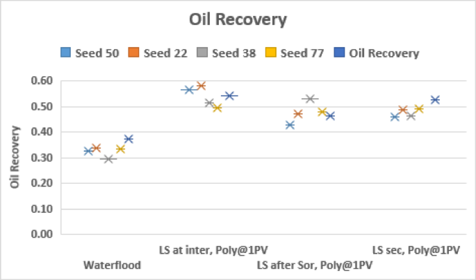
Oil recovery for injection sequences 7–9 and HS waterflood after 3PVs injected for M = 10 across 5 different capillary networks, v = 1 m/day.
The results of Fig. 11 show that when LS brine is injected before polymer solution, the recovery is optimized when the LS brine is injected at an intermediate saturation of HS water.
Polymer injection BEFORE LS Brine
If we change the order and inject polymer before LS, the distribution is shown in Fig. 12.
Final distribution after 3PVs injected for M = 10, v = 1 m/day with Polymer injected prior to LS brine. From Left to right: (a) HS water flood for 3PVs (b) HS water is injected to an intermediate saturation and then flooded with polymer for a total of 1PV. LS brine is then injected simultaneously with polymer for a further 2PVs. (c) HS water is injected to Sor and then flooded with polymer for a total of 1PV. Then LS brine is injected simultaneously with polymer for a further 2PVs. (d) polymer is injected in secondary mode for 1PV, followed by the injection of LS brine simultaneously with polymer for a further 2PVs.
The plots of oil recovery in Fig. 13 clear shows the impact of timing of polymer injection on the amount of oil recovered. The earlier the injection of polymer, the more the oil recovered. Subsequent injection of LS brine yielded approximately 10% additional oil in all 3 cases. This contrasts the observations when LS brine was injected before polymer.
When polymer is injected in secondary mode (Fig. 12(d)), the polymer travels as a stabilized front and has a better areal sweep efficiency and after the introduction of LS brine, capillary resistance is reduced in the higher capillary entry pressure pores that polymer on its own could not displace, causing the fingers to thicken and swell.
With the introduction of polymer at residual saturation of HS water, \(\:{\varvec{S}}_{\varvec{o}\varvec{r}}^{\varvec{H}\varvec{S}}\), the polymer solution mostly travels through established pathways as has been the case with the previous sequences where LS injection was initiated at \(\:{\varvec{S}}_{\varvec{o}\varvec{r}}^{\varvec{H}\varvec{S}}\) – only a few fingers become extended and some additional oil is displaced when LS brine is subsequently introduced, predominantly through the lateral expansion of polymer fronts and improved access to bypassed zones. When polymer is injected at \(\:{\varvec{S}}_{\varvec{o}\varvec{r}}^{\varvec{H}\varvec{S}}\) and LS brine is injected afterwards at 1PV, the oil recovery is higher than when LS brine is injected at \(\:{\varvec{S}}_{\varvec{o}\varvec{r}}^{\varvec{H}\varvec{S}}\) and polymer is injected afterwards at 1PV.
From the observations here, it can be concluded that the injection of LS brine after polymer injection causes the thickening and swelling of fingers leading to additional oil recovery.
Oil recovery and Regime index plots for HS waterflood and injection sequences 10–12 after 3PVs injected. M = 10, v = 1 m/day.
The regime index plot in Fig. 13 shows the switch to a viscous dominated regime after LS brine is injected at 1PV due to the reduction in capillary entry pressures, confirming our earlier observations.
Oil recovery for injection sequences 10–12 and HS waterflood after 3PVs injected for M = 10 across 5 different capillary networks, v = 1 m/day.
From Fig. 14 we can see that the earlier the polymer injection, the more the oil recovered – this is independent of seed number.
Finally, we will examine the results of oil recovery for the injection sequences considered thus far at 10 m/day. Results are shown in Fig. 15.

Oil recovery for all injection sequences 1–12 and different seed numbers at 10 m/day frontal advance velocity, M = 10.
At 10 m/day, When LS brine is injected alone, the results are very similar for secondary LS brine injection and LS brine injection at \(\:{\varvec{S}}_{\varvec{o}\varvec{r}}^{\varvec{H}\varvec{S}}\) and LS injection at \(\:{\varvec{S}}_{\varvec{i}\varvec{n}\varvec{t}\varvec{e}\varvec{r}\varvec{m}\varvec{e}\varvec{d}\varvec{i}\varvec{a}\varvec{t}\varvec{e}}^{\varvec{H}\varvec{S}}\). This is because the high flow rate injection shifts the flow regime to viscous dominated and the impact of capillary pressure is minimized.
When LS brine is injected before polymer, secondary LS brine injection consistently produced the lowest oil recovery across all networks because the viscous fingering at 10 m/day is worse than at 1 m/day, leaving significant oil behind.
When polymer is injected in secondary mode, either together with LS brine or prior to LS brine, the recovery is significantly higher than at 1 m/day.
Experimental validation
To complement and validate the findings on the impact of relative timing between low salinity (LS) brine and polymer injection on oil recovery, a range of core flooding and micromodel experiments from the literature provide strong empirical evidence. These experimental studies offer crucial insights into how wettability alteration, capillary entry pressure reduction, and mobility control mechanisms interact at both the pore scale and laboratory core scale. They also serve to bridge the gap between digital simulation tools and field-level design by physically replicating fluid dynamics in porous media under controlled conditions.
Several studies have demonstrated the critical influence of injection sequence on oil recovery. For instance, Al-Saedi et al. (2019)38 and Yousef et al. (2020)18 showed that injecting LS brine at intermediate water saturations—after partial HS water injection but before breakthrough—enhances oil recovery by shifting wettability and mobilizing previously trapped oil. These findings directly support our simulation results where LS injection prior to HS breakthrough leads to favorable capillary-to-viscous transitions, increased pore accessibility, and more stable front propagation, as captured by our Regime Index formulation.
Further, the synergistic effect of LS brine and polymer injection has been consistently reported in both early and recent literature. Zahid et al. (2012)39 and Wang et al. (2022)19 observed that recovery is maximized when polymer is injected after LS brine due to improved sweep efficiency and delayed breakthrough. Their experiments in sandstone cores found recovery improvements of up to 15–20%, attributed to the combined impact of reduced capillary entry pressures and enhanced mobility control—consistent with our simulated increase in oil recovery in injection sequences involving LS-polymer co-injection at intermediate saturations.
Micromodel experiments by Fadaei et al. (2023)20 provide further visual confirmation. Their work demonstrated that LS brine injected early minimizes viscous fingering, allowing polymer introduced afterward to form more stable displacement fronts and access bypassed zones. This matches the observed improvements in displacement stability and oil mobilization in our network model, particularly in Sequences 5, 6, and 9.
Using advanced CT-imaging, Zhang et al. (2024)21 provided direct evidence of wettability change and phase redistribution during core floods with varying salinity and polymer viscosities. Their results confirmed that LS injection at intermediate saturations improved connectivity and facilitated ganglia mobilization, outcomes which align well with the pressure-gradient-driven displacement shifts and enhanced recovery trends seen in our model.
The importance of injection order was also discussed by Austad et al. (2010)40 who found that LS brine injected after HS waterflooding to residual oil saturation (Sor) produced limited incremental recovery. This is attributed to the formation of established HS flow paths that the LS brine cannot disrupt effectively—a limitation also observed in our simulations, where post-Sor LS injection produced marginal gains due to confinement to existing pathways.
Finally, the regime behavior observed in our simulation—characterized by transitions from capillary to viscous dominance—is supported by experimental results and pressure drop trends reported in Sheng (2014)29. These results emphasize that injecting LS or polymer too late in the flood cycle limits their effectiveness, a point reinforced by the comparative drop in recovery observed in both literature and our later injection sequences.
Taken together, these experimental validations—ranging from core floods to pore-scale visualization—confirm that the sequence and timing of LS brine and polymer injection are pivotal in determining recovery outcomes. Intermediate saturation injection strategies optimize the balance between wettability alteration and mobility control, and the resulting flow regime transitions are captured both experimentally and within our simulation framework. The alignment of these trends across scales and methodologies affirms the robustness of the conclusions presented in this study.
Practical implications and economic considerations
The results of this study have important implications for the design and implementation of enhanced oil recovery (EOR) strategies in the petroleum industry. The observed sensitivity of oil recovery to the relative timing of low salinity (LS) brine and polymer injection suggests that injection sequencing should be treated as a key design parameter, rather than a secondary operational detail. By optimizing the timing—particularly by injecting LS brine prior to polymer or co-injecting at intermediate saturations—operators can maximize the synergistic benefits of wettability alteration and improved mobility control. These findings are especially relevant for waterflooded reservoirs transitioning into tertiary recovery phases, where residual oil saturation is high and traditional polymer floods often suffer from poor sweep efficiency.
From an economic perspective, the combination of LS brine and polymer flooding offers a cost-effective alternative to more complex chemical EOR methods such as surfactant-polymer flooding. As noted by Mohammadi and Jerauld (2012)15, LS brine can significantly reduce polymer adsorption and degradation, thereby lowering the required polymer dosage and improving the efficiency of the polymer bank. This leads to reduced chemical costs and improved injectivity, particularly in sandstone reservoirs with moderate salinity levels. In addition, by enhancing the effectiveness of polymer flooding, LS preconditioning may reduce the total pore volume injected to reach target recovery levels, translating into shorter project lifecycles and reduced water handling costs.
These qualitative conclusions are supported by field-scale studies with economic metrics. For example, Al-Khafaji et al. (2019)38 reported that hybrid LS-polymer injection schemes yielded improved net present value (NPV) and lower cost per incremental barrel compared to polymer-only floods. Similarly, Sheng (2014)13 provided a comparative cost analysis of chemical EOR methods, showing that LS-polymer flooding can achieve favorable economics due to reduced polymer consumption and enhanced recovery efficiency. Stavland et al. (2012)16 also demonstrated that LS brine can improve polymer injectivity and reduce operational costs associated with chemical loss and water management.
Overall, the findings support the use of LS-polymer hybrid flooding as a scalable and economically attractive EOR strategy, provided that injection timing is properly optimized based on reservoir characteristics. Future field pilots and techno-economic evaluations are encouraged to further validate these simulation-based insights.