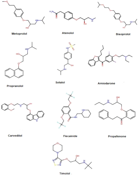
Multi-Criteria Decision Making (MCDM) helps choose the best option when several good choices exist instead of one perfect answer. This research uses specific types of mathematical descriptors, called degree based and neighborhood degree-based topological indices, to analyze drugs that treat arrhythmia. By performing QSPR (Quantitative Structure-Property Relationship) analysis, the study reveals a strong link between these indices and the physical and chemical characteristics of arrhythmia medications like Metoprolol, Atenolol, Amiodarone, Bisoprolol, Propranolol, Sotalol, Carvedilol, Flecainide, Propafenone and Timolol.
This research investigates the chemical properties of substances by employing various topological indices, including the Zagreb, neighborhood harmonic, neighborhood Zagreb, and neighborhood Shilpa-Shanmukha indices. To efficiently pinpoint both the best and worst possible outcomes, a weighted evaluation of these indices will be performed using a decision-making technique like TOPSIS and SAW.
This study also assesses how accurately molecular compounds are described using mathematical techniques. It combines Multi-Criteria Decision Making (MCDM), a method dating back to the 1980s33, with the entropy method to assign weights to various topological indices. The entropy method ensures an impartial assessment of each index’s relevance in predicting drug properties by assigning weights according to data variability. This means that structural features of a drug that show more diversity across compounds will be given greater importance. This systematic approach helps eliminate personal biases, leading to more precise molecular evaluations. The weights are allocated using the formula:
$$\begin{aligned} \sum _{j=1}^{k}w_{j}=1 \end{aligned}$$
Effectiveness of a drug hinges on its physicochemical properties. To identify the most and least desirable characteristics, it’s crucial to examine factors like density, molar volume, and boiling point, flash point, KOC and BFC. For example, a lower density generally leads to better solubility, while a lower melting point makes a drug easier to use. Molar volume plays a role in how a drug crystallizes, with most effective medications typically weighing less than 1000 g/mol. A higher boiling point is beneficial for storage, and the complexity of a drug can impact both how it is administered and its cost.
In Table 13, using the entropy method, we objectively assigned weights to each drug property. This data-driven approach accurately assesses drug characteristics by determining each property’s weight based on its ability to differentiate between drugs, effectively removing any subjective bias.
Ranking of drugs using TOPSIS
We look at each property on its own, then figure out the best choices by seeing how closely they match what we ideally want. Table 11 presents n criteria such as Zagreb indices and harmonic index, and m alternatives i.e, drug structures. To determine the best option, appropriate attribute weights are assigned.
Step 1 Construct an evaluation matrix \((r_{ij})_{m\times n}\) representing where each metric connects with each available choice.
Step 2 Systematize this matrix to get a normalized version \(N=(n_{kj})_ {m \times n}\), Table 12.
\(n_{kj} = \frac{r_{kj}}{\sqrt{\sum _{k=1}^{m} r_{kj}^2}}, \quad \forall k = 1,2,3,\dots ,m \text { and} j = 1,2,3,\dots ,n.\)
Step 3 Let’s break down how we get to our weighted normalized decision matrix, which we are calling \(Y_{ij}\) and you can find in Table 14. We created it by applying the weights that were given to us in a separate Table 13. We will do this by using a specific formula
$$\begin{aligned} \sum _{j=1}^{k}w_{j}=1 \end{aligned}$$
The normalized value is \(y_{kj} = w_j^* \cdot n_{kj} \quad \forall j = 1, 2, 3,…, k\), where \(\sum _{k=1}^n w_k^* = 1\)
Step 4 We are going to determine the best-case scenario ( positive ideal) and the worst-case scenario (negative ideal) for each of our evaluation categories, Table 15. We are going to compare each option to the absolute best possible option (the “ideal” one) and see how much they differ, which is described as, \(Q^+ = \{y_k^+, …, y_j^+\} = \left( \max _{j \in J} \text { or } \min _{j \in J} Y_{kj} \right) Q^- = \{y_k^-, …, y_j^-\} = \left( \max _{j \in J} \text { or } \min _{j \in J} Y_{kj} \right)\)
Step 5 We measure this difference using a method called Euclidean distance, which calculates the “straight-line” distance in multiple dimensions. This gives us a clear number showing how far apart they are. The optimal solution stands apart from the other options because. \(L_{+i} = \sqrt{\sum _{j=1}^{n} (Y_{ij} – Q_{+j})} L_{-i} = \sqrt{\sum _{j=1}^{n} (Y_{ij} – Q_{-j})}\)
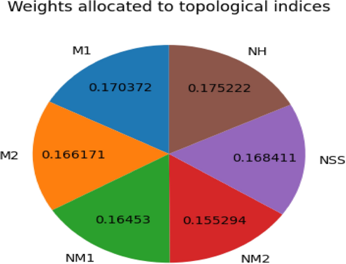
Weights allocated to topological indices.
Figure 5, depicts the weights allocated to the topological indices. The Table 12 shows a decision matrix contrasting different drugs according to the value of different topological indices, such as \(M_1(\varGamma )\), \(M_2(\varGamma )\), \(NM_1(\varGamma )\), \(NM_2(\varGamma )\), \(NSS(\varGamma )\), \(NH(\varGamma )\). Each drug corresponds to particular numerical scores for these indices. For example, Bisoprolol has scores of 0.280068, 0.262623, and 0.264583 for \(M_1(\varGamma )\), \(M_2(\varGamma )\), and \(NM_1(\varGamma )\), respectively, but Atenolol displays lower scores, such as 0.236135 for \(M_1(\varGamma )\). This matrix can not predict if a drug will work, but it does assess how well drugs perform based on their topological characteristics. These characteristics might be related to a drug’s effectiveness in treating conditions like arrhythmia. The scores in the matrix show quantitative differences, which could help in making decisions since specific index scores should correlate with therapeutic success.
Now we compute weights for each neighborhood degree based on topological indices in Table 13, and the weighted decision matrix Table 14.
Step 6 Determine the relative proximity \(B_{i}\) of each alternative answer to the ideal answer Table 15.
\(O_k^\prime = \frac{L_{-k}}{L_{+k} + L_{-k}}, \quad \text {where } 0
\(\text {It is clear that } O_k^\prime = 1 \text { if } Q_k = Q_+ \text { and } O_k^\prime = 0 \text { if } Q_k = Q_-.\)
Step 7 This step involves ordering the reference answers from most similar to the ideal answer to least similar, based on the calculated proximity values \(O_k^\prime\). The references are ranked in descending order of \(O_k^\prime\) Table16.
Our study establishes what constitutes the best and worst choices by examining specific properties that influence how effective medicine is. The ideal best picks comprise high boiling point, polarizability, BCF and KOC. High boiling point can improve drug stability. This means the drug is less likely to break down or degrade at typical storage, A stable drug guarantees that patients get the correct amount of the active ingredient, and the medicine remains effective for its entire shelf life. A drug’s polarizability helps it interact well with different biological molecules and environments, which directly affects its ADME profile (how it’s absorbed, distributed, metabolized, and excreted). Higher value of BCF could reduce the required dosage frequency and potentially enhance therapeutic effect. A medicine with a high value of KOC means that the drug is less likely to leach into water sources, which is a significant environmental and public health benefit.
On the other hand, the ideal worst picks comprise lower values of boiling point, density, and molar volume. Lower boiling point make the compound unstable. A drug which has a very small molecular volume, it might be processed and eliminated from the body quickly. This shortens the time the drug stays active, meaning patients would need to take it more often. Such frequent dosing can make it harder for patients to stick to their medication schedule, potentially leading to inconsistent drug levels in their system which make it worst. When deciding on a drug for arrhythmia, we prioritize characteristics that improve how well it works, giving them more importance in our evaluation. On the other hand, we give less weight to properties that might reduce its effectiveness. This organized method helps us more effectively evaluate and select the best drug candidates for disease treatment.
SAW-based drug ranking
The Simple Additive Weighting (SAW) method, sometimes called the weighted scoring method, is a multi-criteria decision-making tool. It operates by computing a weighted average for each available option. In essence, SAW calculates an overall score for each alternative by multiplying its performance on various criteria by the corresponding importance (weight) of those criteria, and then summing these products. The steps involved in the SAW method compromise ranking procedure are:
Step 1 Create a conclusion matrix Table 11, list the m alternatives and n attributes, identifying the best and worst values for each attribute.
Step 2 Determine the weights by using previously established weighted norms. Subsequently, construct a normalized decision matrix Table 17, using the following formulas:
\(m_{ij} = \frac{j_{kj}}{\max (j_{kj})}\)
\(m_{ij} = \frac{\min (j_{kj})}{j_{kj}}\)
where \(j_{kj}\) is the original value, \(k = 1, 2, 3,…, m\) and \(j = 1, 2, 3,…, n\).
Step 3 Find the value of each replacement by applying the formula. The formula to calculate each substitute’s score is:
\(G_k = \sum _{j=1}^{n} w_j \cdot n_{ij}\)
where \(G_k\) is the weighted sum for substitute i, \(w_j\) is the weight of attribute j. \(n_{ij}\) is the normalized value of substitute i for attribute j, and n is the total number of attributes Table 18.
Our research is really useful for making new medicines, especially for arrhythmia problems. We use special math tools and computer models to figure out how well different drugs might work, Table 19. This approach can help drug companies identify the most promising drug candidates for early testing, which saves them both time and money. Instead of lab-testing every compound, they can use our method to predict which ones are most likely to be effective. This technique is not just for drugs; it can also be useful for environmental chemical analysis or developing new materials.
The normalized decision matrix of different drugs according to topological indices in Table 17 represents the standardized value of the different indices (i.e., \(M_1(\varGamma )\), \(M_2(\varGamma )\), \(NM_1(\varGamma )\), \(NM_2(\varGamma )\), \(NSS(\varGamma )\), and \(NH(\varGamma )\)) of each drug. The normalization process allows the different indices of all the drugs to be on the same scale, so any comparison of the drugs becomes possible on the same level. For instance, “Amiodarone” has the highest normalized value of 1.000000 in the case of \(M_1(\varGamma )\), \(M_2(\varGamma )\), \(NM_1(\varGamma )\), \(NM_2(\varGamma )\), and \(NH(\varGamma )\). Conversely, “Atenolol” possesses comparatively lower normalized value across all the indices; it may thus not be able to perform better in accordance with these topological characteristics. Normalization is a crucial step in preparing data because it puts all the drugs on an equal footing. This means we can compare them fairly, no matter how large or small their original data values were.
Table 18, presents the weighted normalized decision matrix. This updated matrix improves upon the previous one by adjusting the importance of each topological index based on its significance for evaluating the drugs, and then applying these adjusted weights to the normalized values. For example, “Amiodarone” consistently ranks highest across most performance indicators, showing its overall strong effectiveness. This is clear from its high SAW (Simple Additive Weighting) score of 0.997346, confirming it as the top performer, just as expected. “Atenolol” however, ranks last with a comparatively lower SAW value of 0.487281, indicating that it has lower preference when the weighted significance of the indices is used. This weighted system highlights the drugs that perform best on the most important criteria, making it a more precise tool for decision-making.
The final ranking of the drugs according to their SAW scores from the preceding table is presented in Table 19. From the table, it is clear that ”Amiodarone” with a score of 0.997346 rank highest, followed by Carvedilol, and Flecainide with scores of 0.982764 and 0.831580, respectively. This ranking results from the addition of the normalized and weighted scores of each drug, thereby providing a clear comparison. Other drugs like, Metoprolol and Atenolol rank lower, with the last position held by Atenolol. This ranking aids in the informed decision-making process of the most likely best drug.