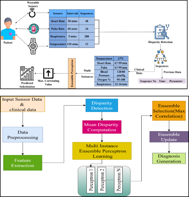
The data analytic model is proposed to sense the clinical data from WS devices that acquire activities vital to humans. This observation takes place periodically, ensembles the clinical data, and detects the function that represents health monitoring in the early stages. In this execution step, the incomplete data are considered and provided incomplete data, which is detected using the data disparity technique. It ensures the prediction model observes the data in the stored dataset and generates the result. This approach is followed up with an MIEPL concept. Figure 1b depicts the workflow of the proposed ADDT architecture.
Input sensor and clinical data are preprocessed to eliminate noise, handle missing values, and normalize for consistency in the described model architecture for the ADDT method. Next, feature extraction extracts relevant and representative features from the processed data. A disparity detection module finds discrepancies and variations across numerous inputs. The system calculates the average deviation of these features using a mean disparity computation. The model begins an MIEPL phase with this disparity information, when many perceptrons simultaneously learn from different data subsets. Independent perceptrons contribute to a prediction pool. The model uses maximum correlation to pick perceptron outputs that agree most to improve accuracy. An ensemble updating method uses performance feedback to fine-tune the selected models. The intelligent decision-making procedure concludes with dependable diagnostic generation from improved ensemble outputs.
The diagnostically important factors, including heart rate variability, blood oxygen saturation trends, glucose fluctuations, and systolic/diastolic patterns, have been analyzed; feature extraction was performed on sensor and clinical data streams before the model was trained. Consideration of clinical relevance and statistical association with labelled diagnosis outcomes informed feature selection. The feature scales were normalized using z-score normalization as part of a preprocessing pipeline that included a moving average filter to decrease noise and clinical-value-based imputation to address missing values. The extracted features \(\:{v}^{{\prime\:}},{a}_{l},{x}^{{\prime\:}},{y}^{{\prime\:}}\) were then evaluated for disparity using the ADDT formulation, with \(\:{M}_{e}\) representing extracted clinical metrics and \(\:D{a}^{{\prime\:}}\) as sensor-derived sequences, these steps ensure that input features are coherent, denoised, and scale-invariant for the perceptron ensemble learning stage.
The evaluation runs through the data analytic method that identifies mean disparity for varying data sequences. The data sequences define the WS data variant and generate the periodic analysis of human health status. This approach evaluates human activities and vitals periodically and makes a diagnosis accordingly. It observes the data from WSs and evaluates them for sequence estimation. This technique detects the disparity in data sequences where the threshold maintenance is defined. The preliminary step is to analyze the incomplete clinical data, which is expressed in the following Equation.
$$\begin{aligned} \nabla & = \mathop \sum \limits_{{v^{\prime} + a_{l} }} \left( {\beta + y’} \right)*\left\{ {\left( {x^{\prime} + Da’} \right) + \left( {Sq*\beta } \right)} \right\}*\mathop \sum \limits_{{y^{\prime}}}^{{a_{l} }} x^{\prime} \\ & + \left( {\frac{\beta }{{\left( {Sq*Da^{\prime}} \right)}}} \right)*\left\{ {\left| {y^{\prime} + \beta } \right|*\left( {Sq + \left( {a_{l} *v^{\prime}} \right)} \right)} \right\} + \mathop \sum \limits_{\beta } Da^{\prime} – i_{p} \\ \end{aligned}$$
(1)
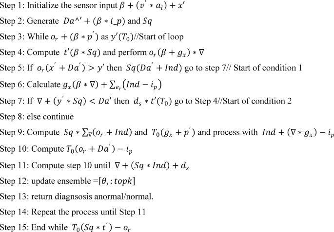
Equation (1) computes the complete clinical data aggregate analysis \(\:\nabla\:\) derived from wearable sensors and helps identify gaps and disparities in clinical data records. This is used to analyze the incomplete clinical data, which refers to the dataset acquired from WS devices. The \(\:{v}^{{\prime\:}}\) are symbolized as detected human activities like walking and sitting, and \(\:{a}_{l}\) as vital signs for heart rate, and temperature. The data storage is\(\:\:Da{\prime\:}\) with healthy records, \(\:\:\beta\:\) is referred to as clinical data parameters like blood pressure, where \(\:\:y{\prime\:}\) is observed as a periodic detection value from the sensor. The sequences of data that are acquired from the sensor are\(\:\:Sq,\) the diagnosis of diseases is\(\:\:x{\prime\:},\) and\(\:\:{i}_{p}\) is labeled as incomplete data points. The term \(\:\sum\:_{\beta\:}D{a}^{{\prime\:}}-{i}_{p}\) Subtract incomplete values to factor in the impact of missing data. The analysis calculates a weighted product of clinical indicators and detected values, helping to estimate data reliability and health trends. From this observation step, the clinical data is acquired from the sensor device\(\:\:\left(\:Sq+Da{\prime\:}\right)*\sum\:_{{i}_{p}}\beta\:\). The examination takes place for the clinical data acquisition and detects incomplete data. The periodic observation is done for the data sequences where the activities are vital. The analysis is done for the data variant where the incomplete sequences are observed from the clinical data and the mapping with previous inputs. The overall representation of ADDT model is provided below:
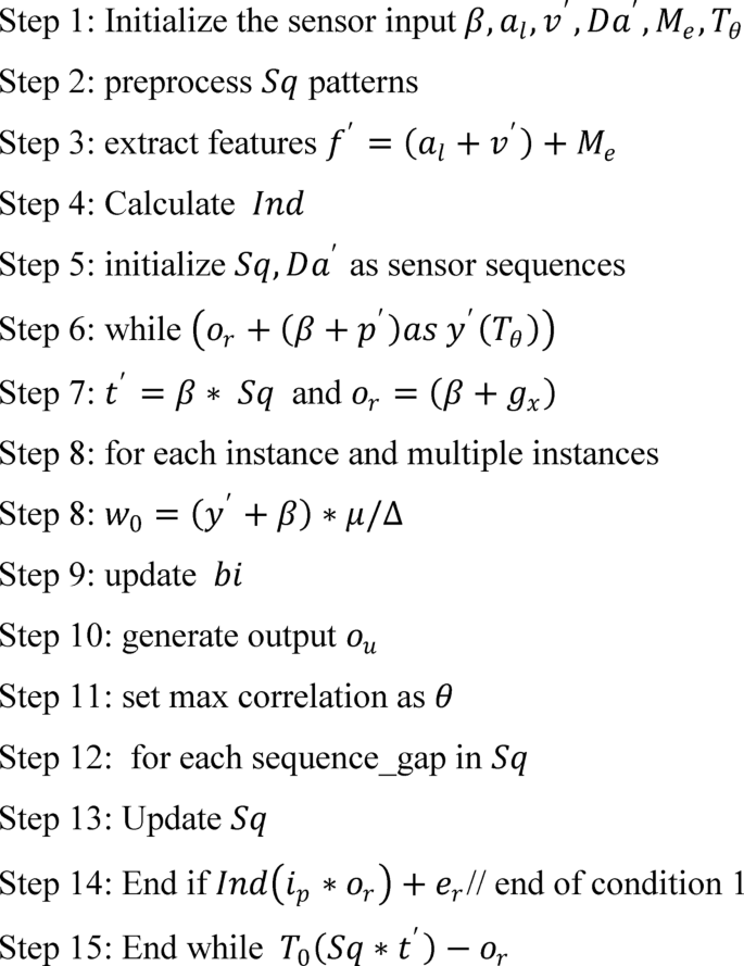
The process begins with initializing the sensor input data, followed by preprocessing to clean and structure the detected patterns. Key features are then extracted to facilitate deeper analysis. A loop mechanism is employed to iteratively evaluate sensor sequences, updating and refining the output at each step. The final output is generated based on maximum correlation and matched patterns, ensuring accurate and efficient sequence recognition.
The computation is done for the clinical data to detect the incomplete data sequences from the dataset. This phase examines the incomplete data that is extracted from the WS. The normal and abnormal values are detected from the attained clinical data, and it is mapped with the dataset\(\:\:\beta\:+\left({i}_{p}*{e}^{{\prime\:}}\right), in this case, greater than 0 resembles normal, or else it represents abnormal. On this basis, clinical data are used to examine the human activities and vital rate, which vary over the desired time interval. This process is carried out by diagnosing the activities and vitals, and it is matched with the dataset and generates the results. The diagnosis is done initially and extracted from the data sequences. Thus, this analysis step indicates the normal and abnormal values extracted from the data sequences acquired from the sensor device. The examination of activities and vitals is observed periodically, derived from the Eq. (2) below, calculates the periodic medical evaluation \(\:{M}_{e}\) analyzing historical and current data from sensor input aids in real-time decision-making.
$$\begin{aligned} M_{e} & = \nabla + \left( {v^{\prime} + a_{l} } \right)*\mathop \prod \limits_{\beta }^{{Sq}} Da^{\prime} + \left( {p^{\prime}*T_{0} } \right) + x^{\prime}*\left[ {\left( {Sq + y^{\prime}} \right)*\nabla } \right]\left[ {\left( {Sq + y^{\prime}} \right)*\nabla } \right] \\ & + \mathop \prod \limits_{{Da^{\prime}}} \left( {v^{\prime}*a_{l} } \right) – i_{p} + \left\{ {\left[ {\left( {T_{0} + Da^{\prime}} \right)*\left( {Sq + e^{\prime}} \right)} \right] + \prod \left( {p^{\prime} + Sq} \right)} \right\}*\left( {\nabla + p’} \right) \\ \end{aligned}$$
(2)
The examination is done for human activities and vital functions, and the data sequences on WSs to capture periodic patient condition updates using real-time and historical data. The products and nested sequences show compounded health risks or events. The use of \(\:{p}^{{\prime\:}}\) as prediction-based features and the clinical data extraction is labeled as\(\:\:e{\prime\:}\) for correlation \(\:\:{T}_{0}\) is represented as detection timestamp. The examination is used to analyze the data extracted from the data sequence periodically\(\:\:\left[\left(Sq+{y}^{{\prime\:}}\right)*\nabla\:\right]\). The periodical data acquisition and the incomplete data from the sequenced sensor devices are evaluated. This data extraction phase is done by diagnosing the medical data and providing the necessary steps. Both the activities and vitals are used to observe the human status periodically. The main concept here is to detect the activities and vital signs periodically, and based on this, necessary action is taken. This process is considered by diagnosing the activities that indicate the data storage and whether it is normal or abnormal. The preprocessing of data for correlation is graphically illustrated in Fig. 2.
Data analysis in the preprocessing stage.
The data analysis rate increases and ensures a higher precision rate by properly detecting the patient’s normal and abnormal activities and vital signs. According to the threshold and update of the patient, the correlation factor\(\:\:\left({M}_{e}+\beta\:\right)\). The detection takes place from the extracted input features, and analysis takes place\(\:\:\left({v}^{{\prime\:}}+{a}_{l}\right)*\nabla\:\). The evaluation is considered for the data sequences associated with decision-making and improving the data analysis rate. The execution occurs by analyzing the clinical data and ensuring the higher threshold value (Fig. 2). The correlation between the activities and vital signs is observed for the data variant observed at different intervals. Based on the different intervals, incomplete data is acquired, and it is determined whether it is normal or abnormal, which is carried out with the prediction step discussed in the section below. Diagnosis uses varying input data and finds diseases at different time intervals. This detection step is used to find the data sequences in data storage and generates the output accordingly. From this observation step, the correlation and prediction are executed and elaborated in the following section, one by one. This case indicates that the clinical data observation for this disparity detection is carried out on the data. The disparity identification \(\:Ind\) used to quantify abnormality or data inconsistency in periodic clinical data is done periodically and expressed in Eq. (3) below. Followed by \(\:{e}_{r}\) as the error rate and residual from the model prediction, also applies \(\:{M}_{e},D{a}^{{\prime\:}},{v}^{{\prime\:}},{a}_{l},{x}^{{\prime\:}},{y}^{{\prime\:}}\) to validate coherence.
$$\begin{aligned} Ind & = \frac{1}{\beta }*\mathop \sum \limits_{\nabla } \left( {y^{\prime} + i_{p} } \right)*\left\{ {\sum \left( {M_{e} + Da^{\prime}} \right)*\left( {v^{\prime} + a_{l} } \right)} \right\} + \left( {e_{r} *p^{\prime}} \right) + T_{0} *\left( {\beta + e^{\prime}} \right) – x^{\prime} \\ & + \mathop \sum \limits_{{M_{e} }} i_{p} *\left( {Da^{\prime} + x^{\prime}} \right)*\left( {x^{\prime} + T_{0} } \right) + Da^{\prime}\left( {M_{e} – y^{\prime}} \right) \\ \end{aligned}$$
(3)
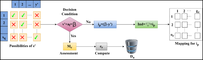
The identification is followed up in the above Equation, which examines the sensor device’s clinical data. This evaluation phase runs on the incomplete data and analyzes the desired value from the sequences. The sequences are considered from the examination, and it is represented as\(\:\:{M}_{e}\), the identification is\(\:\:Ind\), where the extraction is done for the evaluation of normal and abnormal data and acts accordingly. In this execution step, the activities and vital signs are monitored, and where there is coherence with the clinical data and maps with the dataset\(\:\:D{a}^{{\prime\:}}+\left({x}^{{\prime\:}}*\beta\:\right)\). This observation step relies on the disparity of the data and provides the disparity analysis for the coherent clinical data. By evaluating this step, the disparity is considered and provides the output based on the perception learning. This is processed under the prediction state and is observed periodically. The disparity detection flow is illustrated in Fig. 3.
Disparity detection flow illustrations.
The disparity detection process is illustrated in Fig. 3 by interlinking.\(\:\:{y}^{{\prime\:}}\) and\(\:\:Sq\). The aim is that\(\:\:\beta\:\) must balance\(\:\:\sum\:\left({v}^{{\prime\:}},{a}_{l}\right)\) in any\(\:\:{y}^{{\prime\:}}\) provided\(\:\:Sq\) is continuous. Therefore, the failing condition flow estimates the\(\:\:{i}_{p}\) as\(\:\:\left(\beta\:-{y}^{{\prime\:}}\right)\) in any sensed sequence such that\(\:\:Ind\) is the sum of\(\:\:\left(\nabla\:\:\text{a}\text{n}\text{d}\:{i}_{p}\right)\). Surpassing this output, the\(\:\:{g}_{x}\) and\(\:\:{o}_{r}\) mapping occurs for\(\:\:{i}_{p}\) estimation where the correlation between sensor and clinical data occurs. If the above condition is satisfied, then\(\:\:{e}_{r}\) is alone estimated, and the\(\:\:Sq\) is stored in\(\:\:{D}_{a}^{{\prime\:}}\). This\(\:\:{e}_{r}\) if found to be greater than\(\:\:{i}_{p}\), the mapping is further pursued for multiple input instances. In this step, the diagnosis is made for the correlation of the data sequences, and the output is given based on the identification. Identification plays a role in extracting data and finding the disparity in the sequences. If any disparity is detected, the signal is given to the healthcare and the activities and vitals are carried out on an interval basis. This interval of time is considered for the identification of incomplete data, which is mapped with the data\(\:\:{e}_{r}*\sum\:_{Ind}\left({p}^{{\prime\:}}+Da{\prime\:}\right)\). From this observation step, \(\:\left\{\sum\:\left({M}_{e}+D{a}^{{\prime\:}}\right)*\left({v}^{{\prime\:}}+{a}_{l}\right)\right\}\) is examined for the data variant. Based on this identification step, the sequence disparity is coherent with the dataset’s current and existing data. Hereafter, the identification of disparity is computed using the above Equation. The mean disparity is computed through decision-making described in the steps below:
The algorithm works according to the Eq. (4) below, which is generated for the decision-making process.
$$\begin{gathered} d_{s} = \mathop \sum \limits_{\nabla }^{{i_{p} }} Da^{\prime} + \left\{ {\left( {p^{\prime} + T_{0} } \right) + \left( {o_{r} *\beta } \right)} \right\}*\left( {g_{x} + Sq} \right)*\left| {Da^{\prime} + \beta } \right| \hfill \\ + \left( {y^{\prime}*\nabla } \right)*\left( {p^{\prime} + x^{\prime}} \right)*\mathop \sum \limits_{{g_{x} }} \beta + \left( {x^{\prime}*e_{r} } \right) + e_{r} *\left( {\beta + Da’} \right) \hfill \\ \end{gathered}$$
(4)
The decision-making process is represented as\(\:\:{d}_{s}\), \(\:{g}_{x}\) is existing value \(\:\:{o}_{r}\) is the correlation mapping between the current and existing value generated from the medical center. Based on this method, the decision is made on the mean disparity, and the data requirement for the WS sequence is decided. This decision uses multiple substituted and predicted values obtained from previous instances. MIEPL is used in this decision process, where the substitution instances for clinical and previous outcomes are performed. Based on the above steps, the disparity detected for multiple data instances is analyzed in Fig. 4.
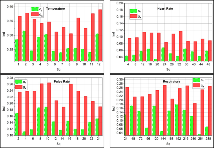
\(\:\:Ind\) analysis for multiple data instances.
The disparity detection is less if it analyzes the incomplete sequence and substitutes medical data. This process indicates the monitoring of the vitals and activities of the patient periodically\(\:\:\left({v}^{{\prime\:}}+{a}_{l}\right)*p{\prime\:}\left({x}^{{\prime\:}}\right)\). In processing this detection, the time interval is considered to observe the disparity and provide the necessary action\(\:\:{e}_{r}\left(\beta\:*{M}_{e}\right)-Ind\). By evaluating this step, detection occurs by mapping carried out with the data storage. The data storage of clinical existing data is mapped and found whether it is normal or abnormal\(\:\:\left({m}_{0}+{b}_{a}\right)\). This analysis phase is done using a prediction method executed in the perceptron learning concept and shows lesser detection of disparity. Real-world wearable sensor data is typically uneven and asynchronously updated, but the ADDT framework is built to handle this and works without regularly spaced data. ADDT continuously compares real-time sensor measurements to clinical or historical values. When missing sequences or asynchronous gaps are found, the system triggers a substitution mechanism to extract the most contextually relevant instances, either temporal trend predictions or clinical data. These substitutions are filtered and weighted using ensemble precision scoring to integrate the most reliable and diagnostically helpful data. This dynamic handling of missing or delayed sequences allows ADDT to function well in extremely irregular real-world monitoring contexts.
Multi-instance ensemble perceptron learning
The proposed MIEPL is unique. It can analyse many sequences of sensor-clinical data (i.e., multi-instances) and produce reliable predictions by merging numerous perceptrons trained on different substitution instances. Our model treats every data sample as a collection of cases instead of the flat feature vector used by conventional perceptron models. This allows us to deal with data samples that fluctuate in time, such as sensor readings and intermittent clinical records. The “multi-instance” method allows the model to learn patterns from clinical data streams partially absent, asynchronous, or unevenly spaced by training and making decisions over similar but not identically structured inputs. By combining the predictions of several perceptron learners that have been trained on various weighted combinations of these input examples, the “ensemble” feature further improves dependability. Each perceptron evaluates the fused feature vector using dynamically assigned weights \(\:{w}_{0}\) from Eq. (7) and threshold calibration \(\:\mu\:\) from Eq. (5) ensures that even inconsistent or incomplete data subsets contribute to an accurate final decision.
The perceptron is a neural learning model that relies on the binary classification method for the attained input data, such as clinical data, and makes decisions accordingly. So, it relies on 0 or 1 cases where the threshold value is generated to observe the threshold value based on the input and weight. The comparison is taken for the weighted input with a threshold value and concludes if the input is greater than it generates the output as 1, or else it is 0. The value of \(\:\mu\:\) is selected through empirical validation using a validation dataset that contains known cases of both normal and abnormal clinical conditions. The \(\:\mu\:\) determines whether the weighted input derived from the sensor-clinical data fusion should be flagged as disperate/ anomalous (1) or acceptable (0). By guaranteeing that only sensor-clinical data inconsistencies that fall significantly below the decision threshold are highlighted, the calibrated µ value increases the accuracy of the ADDT framework and so improves forecast accuracy and system dependability.
$$\:{M}_{e}\left({w}_{0}\right)=\left\{\begin{array}{c}1,\:if\:\beta\:\mu\:\end{array}\right.\:$$
(5)
The above Eq. (5) examines the threshold and maps with the clinical data. The threshold is labeled a\(\:\:\mu\:\), and the weight is\(\:\:{w}_{0}\) where the condition is satisfied with clinical data observation. In this execution step, data sequences are detected to analyze input. From this, the following parameters are discussed in the perceptron learning method.
1.
Extraction of Input features: It evaluates the characteristics and features of input clinical data, where multiple patterns and features are considered using an Eq. (6).
$$\:\nabla\:\left({f}^{{\prime\:}}\right)=\left({a}_{l}+v{\prime\:}\right)+{M}_{e}$$
(6)
The feature of the input data is\(\:\:f{\prime\:}\), which includes the activities and vitals that are examined for the multiple patterns analysis.
2.
Initial Weight: For every initial input, the weights that generate the output are assigned, which is followed up based on the training section where it attains the optimal value given in Eq. (7).
$$\:{\text{w}}_{0}=\left({y}^{{\prime\:}}+\beta\:\right)*\frac{\mu\:}{\nabla\:}\to\:{o}_{u}$$
(7)
The weights are assigned based on the input data, where the output is\(\:\:{o}_{u}\) that results during the training section.
3.
Summation function: A weighted sum of the attained input and distributed according to the respective weights.
$$\:{s}_{f}={w}_{0}\left(\beta\:+{M}_{e}\right)*\prod\:_{y{\prime\:}}\left({p}^{{\prime\:}}+{g}_{x}\right)$$
(8)
The summation function is labeled as\(\:\:{s}_{f}\)where the assignment is carried forward for the clinical data.
4.
Activation function: This is used to observe whether the assigned weight is 0 or 1, which is mapped to the threshold value.
$$\:{t}_{n}={w}_{0}\left(\beta\:\right)*{m}^{{\prime\:}}+\mu\:$$
(9)
The activation function is\(\:\:{t}_{n}\); it generates the weight resulting in either 0 or 1 by mapping with the threshold value, which is discussed in Eq. (5).
5.
Bias Update: This factor is used to predict whether the model is in error, which is observed using a decision-making approach.
$$\:{b}_{i}\left(\nabla\:\right)=\left({t}_{n}*{w}_{0}\right)+{d}_{s}*m{\prime\:}\left(\mu\:\right)$$
(10)
The bias is\(\:\:{b}_{i}\) It is used to predict the value, whether normal or abnormal, and takes place with the decision-making concept.
6.
Final Output: By processing in perceptron learning, output is generated based on the activation function that holds the threshold value, and it is formulated as.
$$\:{o}_{u}={t}_{n}*\left(\nabla\:+\mu\:\right)+\beta\:$$
(11)
The main factor here is the threshold value that indicates the activation function to perform, resulting in the output as 0 or 1. From the above parameter, the work for perceptron learning indicates the steps-wise computation and finds the output with the threshold value. The ensemble learning is diagrammatically depicted in Fig. 5 below.
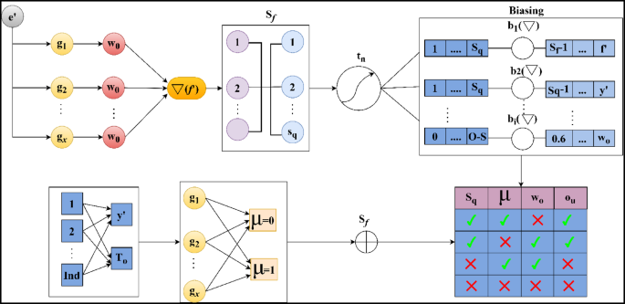
Ensemble perceptron learning depiction for predictive outputs.
The perceptron learning model for predictive outputs of\(\:\:Sq\) substitution is depicted in Fig. 5. The first input is the set of\(\:\:{e}^{{\prime\:}}\) (constant) and\(\:\:{g}_{x}\) (variable) for which independent\(\:\:{\omega\:}_{o}\) is assigned. This\(\:\:{\omega\:}_{o}\) is computed using Eq. (7) to ensure\(\:\:{S}_{f}\) meets the constraint\(\:\:\left({a}_{l}+{v}^{{\prime\:}}\right)\). If the constraint is satisfied, then the possibility of\(\:\:{e}^{{\prime\:}}\) is higher than the previous\(\:\:{g}_{x}\). Therefore, \(\:{d}_{s}\) for\(\:\:{M}_{e}\left({\omega\:}_{o}\right)\) is alone computed for\(\:\:{b}_{i}\left(\nabla\:\right)\) process. If these computations are sufficient for prediction, then the ensembles of\(\:\:{g}_{x}\) are confined to augment\(\:\:{e}^{{\prime\:}}\). Else,\(\:\:Ind\) was observed under\(\:\:{y}^{{\prime\:}}\)and\(\:\:{T}_{o}\) are used to verify\(\:\:{S}_{f}\) using\(\:\:\mu\:=0\) (minimum) and\(\:\:\mu\:=1\) (maximum) threshold outcomes. Therefore, the consecutive computation of the predictive output relies on\(\:\:Sq\) (presence) to ensure high predictive outputs are achieved. The substitution accuracy is graphically analyzed from this learning model as in Fig. 6.
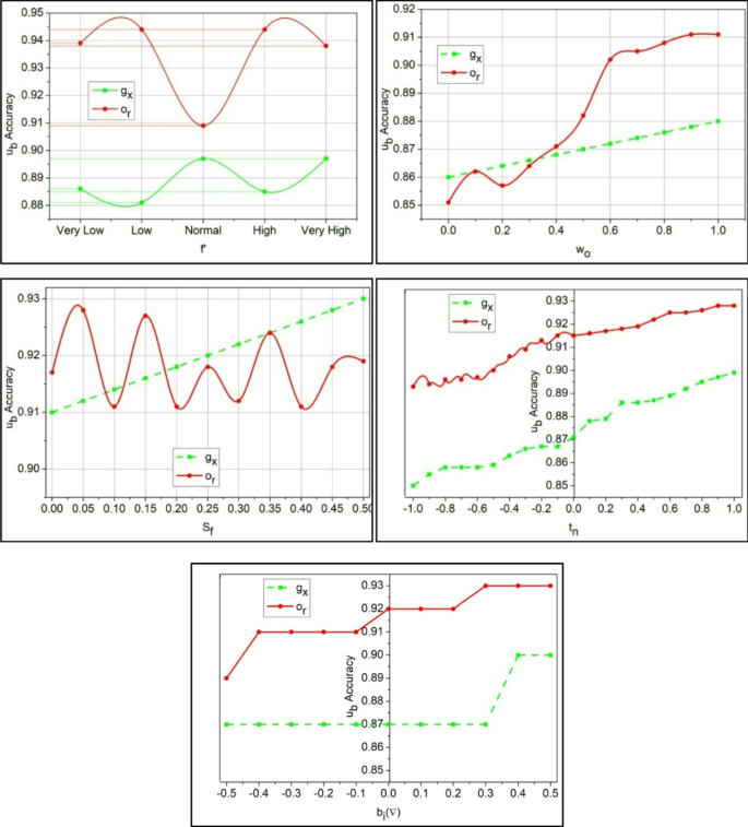
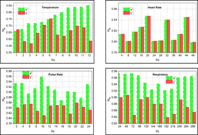
Substitution of\(\:\:{u}_{b}\) accuracy analysis.
The substitution accuracy shown in Fig. 6 is higher, which indicates the WSD for the data variant and observes the mapping for the vital activities.\(\:\:\left({v}^{{\prime\:}}+{a}_{l}\right)*\sum\:_{{M}_{e}}\left({y}^{{\prime\:}}+\beta\:\right)\). This detection occurs periodically, and data storage is used to identify the disparity. This substitution value is used to provide the threshold value, and it generates higher precision\(\:\:\mu\:>{u}_{b}\left(\gamma\:\right)+Sq\). Processing this step indicates the detection of normal and abnormal clinical data. The detection of maximum correlation is presented in the following algorithm.
Correlation of sensor input
The correlation is used to find a similar value from the clinical data and to observe a better diagnosis of human activities and vital signs. If the correlation is the same or equal, no emergency is observed, whereas if it is higher or lower, the emergency threshold is considered.
The above algorithm states the correlation factor for the clinical data and finds the mapping with the threshold value, which is equated in the following derivative.
$$\begin{aligned} o_{r} & = \mathop \sum \limits_{\beta }^{{p’}} \left( {\mu + d_{s} } \right)*a_{g} + \left( {Da^{\prime}*e_{r} } \right)*\left\{ {\left[ {\left( {p^{\prime} + T_{0} } \right) + \left( {\gamma – \beta } \right)} \right] – e_{r} } \right\} \\ & + \mathop \sum \limits_{{w_{0} }} \left( {g_{x} + t^{\prime}} \right)*\left[ {\left( {b_{i} + w_{0} } \right)*\beta } \right] – e_{r} + \left( {Da^{\prime}*f^{\prime}} \right)~ \\ \end{aligned}$$
(12)
The correlation is derived from the threshold and decision-making process, which detects normal and abnormal signals from the sensor. The variables\(\:\:{m}_{0}\:\text{a}\text{n}\text{d}\:{b}_{a}\) are symbolized as normal and abnormal,\(\:\:\gamma\:\) is represented as a prediction. The substitute data is labeled as\(\:\:{u}_{b}\). The sequence error analysis is presented in Fig. 7 based on the correlation process.
Sequence error analysis post the correlation.
The sequence error is less if it reaches below the threshold value, and examines the mapping with the extracted vitals and activities using\(\:\:{t}^{{\prime\:}}\left(\beta\:+{g}_{x}\right)+{d}_{s}\). From this detection phase, identification is carried out to determine whether it is maximum or minimum. In executing this, a disparity detection is performed.\(\:\:{p}^{{\prime\:}}\left({T}_{0}+{y}^{{\prime\:}}\right)*\sum\:_{{e}_{r}}\gamma\:\). This observes the periodic identification of data\(\:\:\left(Ind+\beta\:\right)*\gamma\:-{e}_{r}\left({g}_{x}\right)\). Considering that these error sequences occur due to incomplete data, it is observed that this indicates the assignment of weights for the input (Fig. 7). Following this method, the prediction is followed up with the upcoming algorithm.
Sequence value prediction
The prediction is followed up by mapping with the attained threshold value, where the decision is made accordingly to the variant data analysis. This approach indicates the data sequences and finds the normal and abnormal signals. The algorithm below is used to define the prediction.
The prediction is followed up for the clinical data, where the mapping is followed up by incomplete data observation, represented in the following Equation.
$$\begin{aligned} \gamma & = \left[ {\left( {T_{0} \left( {\mu > m_{0} } \right)} \right)Da’} \right] + f^{\prime}\left( {o_{u} + Sq} \right)*T_{0} \\ & + \mathop \sum \limits_{{Da^{\prime}}} \left( {e_{r} + t_{n} } \right)*f^{\prime} – \left( {g_{x} + t_{n} } \right)*\beta + \left( {i_{p} *o_{u} } \right) + Ind*Da’ \\ \end{aligned}$$
(13)
The prediction is done for the existing value from the clinical data observation, which executes the identification of data sequences progressing in the above Equation. Hereafter, the diagnosis coalition between clinical and update is done periodically for the new precision level that has been identified.
$$\:{x}^{{\prime\:}}\left(\beta\:\right)=Ind\left({i}_{p}-{x}^{{\prime\:}}\right)-{b}_{a}-{m}^{{\prime\:}}\left(\gamma\:\right)*\mu\:+D{a}^{{\prime\:}}\left(Sq*{y}^{{\prime\:}}\right)-{e}_{r}$$
(14)
The above Equation is derived for the analysis of threshold value generation, generating higher precision values identified with the decision-making approach. This process indicates the periodical observation method for clinical data. It correlates with the existing value, finding whether it is a substitute or incomplete data, and based on this, precision is enhanced. Perceptron Learning is used to perform substitution instances for clinical and previous outcomes. The ensemble perceptron selects the maximum clinical value correlating sensor data to ensure high sequence prediction. The ensembles are updated based on the highest precision-based WS values for diagnosis. This diagnosis-focused coalition between clinical and predicted WS values is updated periodically for the new precision levels identified.