The West Karun region, located in the western part of Khuzestan Province, is one of Iran’s most notable petroleum zones, encompassing several large and small oil fields. This region contains three major oil fields along with ten smaller ones, with total oil reserves estimated to exceed 67 billion barrels of oil in place. The proximity of these oil fields to key water bodies, including the Karun and Karkheh Rivers as well as the Hoor Al-Azim wetland, underscores the critical importance of environmental considerations in this area. The ecological sensitivity of the surrounding aquatic ecosystems highlights the necessity of continuous monitoring and assessment of potential pollutants and emissions resulting from oil extraction and production activities. The extent of the study area is shown in Fig. 1 (This map was prepared using ArcGIS software (version 10.8, developed by Esri, Redlands, California, USA) for use in this study).
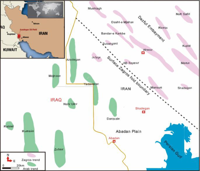
Study area (This map was prepared using ArcGIS software, version 10.8).
Drilling wastewater treatment process
In the drilling wastewater treatment process, the generated effluent collected in designated ponds, where its physicochemical properties are measured. A detailed physicochemical characterization of the drilling wastewater was compiled based on laboratory reports from the treatment facilities in the West Karun oilfields. Table 1a presents the range, average, and standard deviation of key parameters such as COD, BOD₅, TOC, color, nitrogen compounds, TPH, and metals. These values provide insight into the complexity and variability of the effluent matrix, which is crucial for modeling and treatment optimization. In a few cases, data for parameters such as COD and trace metals were not consistently available in daily records. However, these gaps were compensated using laboratory-verified composite samples or averaged values obtained from batch monitoring over representative time periods. The exclusion of these occasional data gaps did not affect the modeling process, as sensitivity analysis confirmed the dominance of other variables (pH, hardness, TSS, Cl⁻) in determining coagulant dosing.
Subsequently, jar tests are conducted to determine the optimal dosage of coagulants and flocculants under various conditions, allowing for the selection of the most effective treatment parameters. In the treatment unit, commonly referred to as the dewatering unit, polyaluminum chloride (PAC) is used both as the coagulant and flocculant. These chemicals are injected using specialized, adjustable pumps. After discharge from the dewatering unit into a secondary holding tank and allowing sufficient time for the coagulation process to complete, the effluent is transferred to a solid-liquid separation system. Following further analysis of turbidity, TSS, and chemical parameters, the treated water is evaluated for reuse (Fig. 2).
One of the most time-consuming and limiting steps in this process is the implementation of jar tests. Therefore, the present study is based on the replacement of this conventional step with artificial intelligence (AI) techniques to enhance efficiency and optimize treatment operations.
Variables study
In this study, the primary dependent variables are the concentrations of polyaluminum chloride (PAC) and anionic polyacrylamide, both of which serve as key chemical agents in the coagulation–flocculation treatment process. The effectiveness of these agents is evaluated based on their impact on the secondary dependent variables: turbidity and total suspended solids (TSS) in the treated effluent.
The independent variables consist of key physicochemical properties of the influent wastewater, which are expected to influence the treatment efficiency. These include total hardness (mg/L as CaCO₃), pH, and chloride concentration (mg/L). These input parameters are measured prior to treatment and serve as the basis for determining optimal coagulant and flocculant dosages through both experimental testing and predictive modeling.

Drilling wastewater treatment process flowchart.
ModelingPrincipal component analysis
Principal Component Analysis (PCA) is a widely applied multivariate statistical technique primarily used for reducing the dimensionality of complex datasets. The core objective of PCA is to transform a large set of possibly correlated explanatory variables into a smaller set of uncorrelated variables known as principal components. This not only simplifies the structure of the data but also mitigates multicollinearity issues commonly encountered in high-dimensional analyses17.
PCA is especially useful when the input vector contains many variables that are strongly correlated. Through this method, the input components are transformed into orthogonal (uncorrelated) variables, ensuring that each new component captures unique information. Additionally, these orthogonal components are ordered based on the amount of variance they explain in the dataset, with the first few components accounting for the most significant variations. Finally, PCA facilitates the removal of components that contribute minimally to the overall variance, thereby simplifying the dataset without a substantial loss of information18.
Data classification
For the purpose of training the artificial neural networks, a percentage-based distribution of the total dataset (n = 193 samples) was defined. The entire dataset was divided into three subsets: approximately 70–80% of the data was allocated for training, 10–20% for testing, and the remaining 10% was used for validation. This classification ensures that the model is trained effectively while also allowing for robust evaluation and generalization of its predictive performance. To address the risk of overfitting due to the limited sample size, 5-fold cross-validation was implemented for each model. The training process was repeated five times with different data partitions, and mean performance metrics (R, RMSE, NSE, and AIC) along with standard deviations were calculated. This approach ensured robustness and helped assess model stability and generalization ability.
Data normalization
The collected data for the variables exhibited a wide and non-uniform range of values, which is an inherent characteristic of the process. However, during model training, such variability in the data can lead to scattered distributions that increase the convergence time of the learning algorithm and, in some cases, result in suboptimal performance. To address this, data scaling was applied to convert the variables into a uniform range by normalizing the original values to a scale between 0 and 1. This normalization was performed using the minimum and maximum values of each variable, ensuring the preservation of proportional relationships within the dataset without affecting the integrity of the data (Eq. 1)19.
$$\:\text{X}\text{n}\text{o}\text{r}\text{m}\text{a}\text{l}\text{i}\text{z}\text{e}\text{d}=\:\frac{\text{X}-\text{X}\text{m}\text{i}\text{n}}{\text{X}\text{m}\text{a}\text{x}-\text{X}\text{m}\text{i}\text{n}}$$
(1)
Select the algorithm
The selection of AI models in this study was guided by their performance in prior water treatment studies and their ability to model nonlinear relationships. Specifically, Random Forest (RF) and Extreme Learning Machines (ELM) were chosen for their robustness in handling tabular data with nonlinear interactions and minimal preprocessing requirements. The RNN and PSO-RNN were included for exploratory purposes based on their success in other environmental prediction tasks, despite the non-sequential nature of our dataset. While RNNs are traditionally designed for temporal or sequential data, some studies have explored their application to complex static datasets where underlying patterns may mimic latent dependencies or contextual transitions. Nevertheless, we acknowledge that more classical approaches such as multiple regression, support vector machines (SVM), or feedforward neural networks may be more appropriate for this type of tabular data20.
Recurrent neural network
This technique features an additional memory state for neurons to share similar parameters. RNN is a type of Feedforward Neural Network (FFNN) in which information is transmitted from the input layer to the output layer. The output of a specific layer is stored and connected to the input for the purpose of predicting the output. The RNN utilizes its internal state to process input sequences of varying lengths. The use of this network is typically in Long Short-Term Memory (LSTM), which includes three gates (input, output, and forget gates) to calculate the hidden state. Although RNNs are commonly used in sequential or time-series applications, they can also capture complex nonlinear dependencies in tabular datasets, especially when input variables exhibit latent interactions or indirect temporal correlations (e.g., changes in influent quality over sequential batches). In this study, RNN was used to investigate its capacity for generalization in scenarios with potential hidden sequential dynamics in operational datasets21.
Hybrid recurrent neural network and particle swarm optimization
RNNs, due to their feedback connections, are ideal for spatiotemporal information processing problems such as real-time data prediction, dynamic system modeling, and process control. However, the presence of feedback connections makes training RNNs significantly more challenging compared to static neural networks. Therefore, developing a new automated algorithm to determine the appropriate structure and parameters from input-output data is essential. Alternative approaches such as Genetic Algorithms (GA), Particle Swarm Optimization (PSO), and their hybrid methods have been successfully employed to evolve RNNs. However, most of these methods evolve the parameters (e.g., weights) of RNNs without considering the structural optimization of the networks22. As a parallel algorithm, PSO operates faster and with less structural complexity compared to other algorithms. PSO has been used to optimize the RNN training process, accelerating the convergence rate of the training and preventing the network from being trapped in local optima23.
Extreme learning machine
Extreme Learning Machine (ELM), proposed by Huang, is a simple and efficient feedforward neural network with a single hidden layer. As a type of neural network, ELM is primarily used for regression, pattern recognition, and classification tasks. Notably, this algorithm requires only the specification of the number of hidden layer nodes, after which it can achieve an optimal solution without the need to adjust input weights or be influenced by the hidden layer. Therefore, ELM is suitable for almost all nonlinear activation functions and does not require tuning of input weights or impact factors. ELM offers better generalization capability and significantly reduced training time. In recent years, many improved algorithms have been developed for ELM, and numerous studies have explored its application in wastewater treatment systems, such a Primary lateral sclerosis (PLS-based ELM) and ensemble ELM models.
Random forest network
This technique constructs Decision Trees (DTs) based on data samples, performs prediction using each individual tree, and ultimately selects the optimal solution through a voting mechanism. The advantage of using a Random Forest is that it reduces overfitting by averaging the results of multiple decision trees. As illustrated in the figure, random samples are selected from a given dataset, and a decision tree is built for each sample. The output from each decision tree is then obtained. The next step involves applying a voting process to all predicted outcomes, with the final prediction being the one that receives the majority of votes. This method exhibits significantly lower sensitivity to the training data by constructing a random forest through the creation of new datasets from the original data and training a decision tree on each bootstrap sample. It is important to note that a random subset of features is selected for each tree and used in the training process. Bootstrapping ensures that the same data is not used for every tree, thereby enhancing the model’s robustness to variations in the original training dataset24,25.
Evaluation criteria
To evaluate model performance comprehensively, both correlation-based and error-based metrics were used. The Pearson correlation coefficient (R) reflects the strength of linear association between predicted and observed values but does not account for magnitude of prediction errors. In contrast, RMSE and NSE provide a scale-sensitive measure of prediction accuracy. Therefore, a high R value may still co-occur with a high RMSE, especially if the model captures general trends well but fails to predict outliers or extreme values accurately. In this study, models with high R and low RMSE/NSE are considered reliable, while large discrepancies between these metrics indicate potential overfitting or lack of generalization.
Correlation coefficient
The value of correlation coefficient (R) represents the correlation obtained between the network outputs and the target values; an R value of 1 indicates a perfect fit. (Eq. 2) corresponds to the calculation of the correlation coefficient of the network26.
$$\:\text{R}=\frac{\sum\:_{\text{i}=1}^{\text{N}}({\text{x}}_{\text{i}}-\stackrel{-}{\text{x}})({\text{y}}_{\text{i}}-\stackrel{-}{\text{y}})}{\sqrt{\sum\:_{\text{i}=1}^{\text{N}}{({\text{x}}_{\text{i}}-\stackrel{-}{\text{x}})}^{2}}\sum\:_{\text{i}=1}^{\text{N}}{({\text{y}}_{\text{i}}-\stackrel{-}{\text{y}})}^{2}}$$
(2)
Xi, Actual value (target), xˉ, predicted value by the model, yi, mean of actual values, yˉ, mean of predicted values, ∑, summation over all data points and R, correlation coefficient.
Root mean square error
The Root Mean Square Error (RMSE) (Eq. 3) is used as a performance metric to compare the prediction capability of an artificial neural network trained on each dataset. When predictive performance among different predictors is evaluated, RMSE serves as a descriptive and informative indicator27.
$$\:\text{R}\text{M}\text{S}\text{E}=\frac{1}{\text{n}}\sqrt{\sum\:_{\text{i}=1}^{\text{n}}{\left({\text{y}}_{\text{i}}-{\text{t}}_{\text{i}}\right)}^{2}}$$
(3)
n, total number of data points (samples), yi, predicted value for the sample, ti, true (actual/target) value for the sample.
Nash-sutcliffe efficiency (NSE)
The NSE is used to assess the predictive power of hydrological models and is defined as (Eq. 4)28:
$$\:NSE=1-\left(\frac{\sum\:({Y}_{i}-{\text{Ŷ}}_{i}{)}^{2}}{\sum\:({Y}_{i}-{\text{Ŷ}}_{mean}{)}^{2}}\right)$$
(4)
where Yi is the observed value, Ŷi is the predicted value, and Ymean is the mean of observed values. An NSE of 1 indicates perfect prediction, while values below zero suggest the model performs worse than the mean of observations.
Akaike information criterion (AIC)
The AIC provides a means of model selection considering both the goodness of fit and model complexity. It is calculated as (Eq. 5)29:
$$\:AIC=2k-2\text{l}\text{n}\left(L\right)$$
(5)
where k is the number of parameters in the model and L is the maximum value of the likelihood function for the model. Lower AIC values indicate better model performance.
Data analysis
MATLAB is a matrix-based software tool well-suited for performing mathematical computations in engineering and basic sciences. Its widespread adoption in both academic and industrial communities is due to its high computational efficiency, ease and speed of programming, matrix-oriented operations, rich library of mathematical functions, and the availability of practical toolboxes. The Neural Network Toolbox in MATLAB provides tools for designing, implementing, visualizing, and simulating neural networks. It also supports a wide range of proven network paradigms and includes graphical user interfaces (GUIs) that allow users to design and manage neural networks in a highly intuitive manner. In this study, MATLAB was utilized for coding and executing the selected algorithms30.