The main procedures for producing PDSI_CMIP6 are outlined in Fig. 2. We obtained monthly meteorological and hydrological outputs from 11 climate models in CMIP6 under various emission scenarios. We utilized the self-calibrated PDSI algorithm, which presented superior performance in spatial comparabilities than conventional PDSI28,29. All calculations were conducted on a grid scale for each model individually, after which the results were integrated into an ensemble. The calculated PDSI values were compared with soil moisture simulations for validation. Finally, a spatiotemporal analysis of the derived PDSI under climate change was conducted as an illustrative example, revealing the hydrological response to future warming. Further details about the methods and data are provided in the following sections.
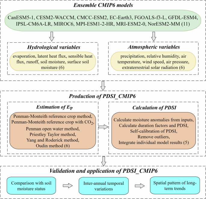
Schematic of the generation of PDSI_CMIP6. Values within the brackets represent the number of datasets, variables, or methods.
CMIP6 simulations
Multiple variables were directly derived from CMIP6 climate model outputs to facilitate the calculations of PDSI, containing six hydrological variables and six meteorological variables. The six hydrological variables include evaporation (variable name: evspsbl), latent heat flux (variable name: hfls), sensible heat flux (variable name: hffs), runoff (variable name: mrro), soil moisture (variable name: mrso), and surface soil moisture (variable name: mrsos). Additionally, the six meteorological variables include precipitation (variable name: pr), relative humidity (variable name: hurs), air temperature (variable name: tas), wind speed (variable name: sfcWind), air pressure (variable name: ps), and extraterrestrial solar radiation (variable name: rsdt)30. These variables were retrieved monthly for the historical period (1850–2014) and projected future period (2015–2094) under four climate change scenarios: SSP1-2.6, SSP2-4.5, SSP3-7.0, and SSP5-8.5, representing different socio-economic pathways and emissions trajectories. Specifically, SSP1-2.6, SSP2-4.5, SSP3-7.0, and SSP5-8.5 correspond to sustainable development, middle-of-the-road development, regional rivalry, and fossil-fueled development, respectively, with projected radiative forcing levels of 2.6, 4.5, 7.0, and 8.5 W/m² by the year 210031. The selection of models, study periods, and future scenarios is intended to maximize data availability. Eleven models were selected, as they are the only ones providing the required 12 variables from 1850 to 2094 under all scenarios (Table 1). These models are managed by different institutions and have varying spatial resolutions ranging from 0.7° (EC-Earth3) to 2.8° (CanESM5-1). For models from the same institution, only the one with the highest spatial resolution (e.g., MPI-ESM1-2-HR vs. MPI-ESM1-2-LR), the most advanced representation (e.g., CMCC-ESM2 vs. CMCC-CM2-SR5), or the standard configuration (e.g., EC-Earth3 vs. EC-Earth3-Veg) is retained to avoid bias within the ensemble. The model outputs were interpolated to a consistent 1° resolution using the first-order conservative remapping method to embed the results32.
Quantification of EP
To test how EP estimates affect the PDSI calculation, we estimated EP using six different approaches, including the Penman-Monteith reference crop (PM-RC) equation33, the Penman-Monteith reference crop considering the plant response to CO2 changes (PM-RC-CO2)22, the open water Penman equation (Penman-OW)34, the Priestley-Taylor model (PT)35, the Yang and Roderick model (YR)36, and the Oudin model37.
The PM-RC is the standard approach for estimating water consumption from reference crop under non-water-limited condition recommended by the Food and Agriculture Organization of the United Nations, which is expressed as:
$${E}_{{\rm{P}}}=\frac{\Delta \cdot \left({R}_{{\rm{n}}}-G\right)/\lambda +\gamma \cdot \frac{900}{T+273}{\cdot u}_{2}\cdot \left({e}_{{\rm{s}}}-{e}_{{\rm{a}}}\right)}{\Delta +\gamma \cdot \left(1+0.34{\cdot u}_{2}\right)}$$
(1)
where Δ is the slope of the saturation vapor pressure curve (kPa·°C−1), γ is a psychrometric constant (kPa·°C−1), u2 (m·s−1) is the wind speed at the 2-meter level above the ground, es and ea are the saturation and actual vapor pressure (kPa), respectively. Rn is the net radiation at the crop surface (MJ·m−2·d−1) and G is soil heat flux density. The difference between Rn and G (i.e., Rn − G) is equivalent to the sum of the latent and sensible heat fluxes. \(\lambda \) is the latent heat of vaporization (MJ·kg−1).
However, a recent study suggested that the neglected plant response to elevated CO2 would cause overrated EP from the original PM-RC algorithm, resulting in inaccurate PDSI estimation. A new variant of the PM-RC method has been proposed to account for the plant response of CO2 changes (i.e., PM-RC-CO2)22, which is also applied for the EP estimation of PDSI_CMIP6:
$${E}_{{\rm{P}}}=\frac{\Delta \cdot \left({R}_{{\rm{n}}}-G\right)/\lambda +\gamma \cdot \frac{900}{T+273}{\cdot u}_{2}\cdot \left({e}_{{\rm{s}}}-{e}_{{\rm{a}}}\right)}{\Delta +\gamma \cdot \left\{1+{u}_{2}\cdot \left[0.34+2.4\cdot {10}^{-4}\cdot \left([{\rm{Ca}}]-300\right)\right]\right\}}$$
(2)
where [Ca] is the concentration of the atmosphere CO2 (ppm).
The Penman-OW model estimates EP as34:
$${E}_{{\rm{P}}}=\frac{\Delta \cdot \left({R}_{{\rm{n}}}-G\right)+\gamma \cdot 6.43\cdot \left(1+0.536{\cdot u}_{2}\right)\cdot \left({e}_{{\rm{s}}}-{e}_{{\rm{a}}}\right)}{\lambda \cdot (\Delta +\gamma )}$$
(3)
Different from the Penman-type methods, the PT method does not provide an explicit expression of the aerodynamic term, and calculates EP as35:
$${E}_{{\rm{P}}}=\alpha \cdot \left({R}_{{\rm{n}}}-G\right)\cdot \frac{\Delta }{\lambda \cdot (\Delta +\gamma )}$$
(4)
where \(\alpha \) is the Priestley-Taylor coefficient, and is taken as a fixed value of 1.26 (Priestley-Taylor coefficient).
The YR method adpots a similar form with PT but an improved parameterization of the Bowen ratio36:
$${E}_{{\rm{P}}}=\frac{\Delta }{\lambda \cdot (\Delta +\beta \cdot \gamma )}\cdot \left({R}_{{\rm{n}}}-G\right)$$
(5)
where \(\beta \) is a dimensionless coefficient of 0.24.
The Oudin model is a tempearture-based EP model and is expressed as37:
$${E}_{{\rm{P}}}=\frac{{R}_{{\rm{e}}}}{\lambda \cdot \rho }\cdot \frac{T+5}{100},\,\text{if}\,T+5 > 0$$
(61)
$${E}_{{\rm{P}}}=0,\text{if}\,T+5\le 0$$
(62)
where Re is the extraterrestrial radiation (MJ · m−2 · d−1), and ρ is the density of water (kg · m−3).
Estimation of PDSI
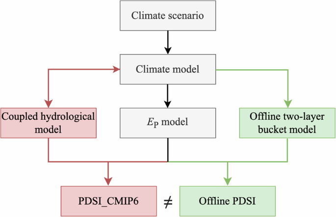
The original PDSI relies solely on precipitation and EP to simulate regional water balance using a simple two-layer bucket water balance model, which estimates evaporation (E), recharge to soils (R), runoff (RO), and water loss to the soil layers (L)18. These modeled hydrological variables are then used to derive a standardized index (i.e., PDSI) that measures the departure of the current hydrological status from its climatological mean. However, the original two-layer bucket model has been criticized for being oversimplified, lacking representations of many processes such as snow/frozen soil and vegetation that affect hydrological dynamics22. More importantly, the estimated hydrological variables from this two-layer bucket model differ from those estimated by climate models, leading to internal inconsistencies between the projected PDSI and climate models. To address these issues, we disregarded the hydrological calculations embedded in the original PDSI model and instead relied on direct hydrological outputs from climate models for the calculation of PDSI23.
Potential values for different water balance fluxes, including potential recharge to soils (RP), potential runoff (ROP), and potential water loss to the soil layers (LP), are defined following EP to measure the deviation from the climatology. The available water capacity (AWC), considered as the soil moisture maximas in different models, is required to describe soil dynamics. The climatically appropriate for existing conditions (CAFEC) values are subsequently defined as the product of the potential values and corresponding climatology coefficients, denoted as α:
$${\alpha }_{{\rm{X}}}=\frac{\bar{X}}{{\bar{X}}_{{\rm{P}}}}$$
(7)
where \(\bar{X}\) and \({\bar{X}}_{{\rm{P}}}\) represents the long-term average of actual and potential values of various water balance components. In particular, the CAFEC precipitation (\(\hat{P}\)) represents the amount of precipitation needed to maintain a normal soil moisture level:
$$\hat{P}={\alpha }_{{\rm{E}}}\cdot {E}_{{\rm{P}}}+{\alpha }_{{\rm{R}}}\cdot {R}_{{\rm{P}}}+{\alpha }_{{\rm{RO}}}\cdot {{RO}}_{{\rm{P}}}-{\alpha }_{{\rm{L}}}\cdot {L}_{{\rm{P}}}$$
(8)
The difference between actual precipitation and \(\hat{P}\) is given as the moisture departure (D):
A monthly climatic characteristic coefficient (\({K}_{i}^{{\prime} }\)) is applied to consider different meanings of \({D}_{{\rm{i}}}\) in different regions:
$${K}_{i}=1.5{\cdot \log }_{10}\cdot \left(\frac{\frac{{\bar{{E}_{{\rm{P}}}}}_{i}+{\bar{R}}_{i}+{\overline{{RO}}}_{i}}{{\bar{P}}_{i}+{\bar{L}}_{i}}+2.8}{{\bar{D}}_{i}}\right)+0.5$$
(101)
$${K}_{i}^{{\prime} }=\,\frac{17.67}{\mathop{\sum }\limits_{i=1}^{12}{\bar{D}}_{i}\cdot {K}_{i}\,}{\cdot K}_{i}$$
(102)
where the subscript i denotes the status in the month i (from 1 to 12). The PDSI index can be subsequently calculated as:
$${{Z}_{i,j}=D}_{i,j}\cdot {K}_{i}^{{\prime} }$$
(111)
$${{PDSI}}_{i,j}=p\cdot {{PDSI}}_{i-1,j}+q\cdot {Z}_{i,j}$$
(112)
where the subscript j denotes the status in the year j from 1850 to 2094, with the whole period used for coefficients calibration. p and q are the duration coefficients to determine the sensitivity of PDSI to moisture anomaly (\({Z}_{i,j}\)) and its auto-correlation. They are considered as 0.897 (p) and 1/3 (q) based on linear slopes between the length and severity of the most extreme droughts observed in Kansas and Iowa, United States38. However, the application of traditional PDSI is constrained by limited spatial comparability, which has been improved via a self-calibration procedure28,29. It re-fits a linear regression model using the original PDSI scores and derives a new set of parameters p and q for each grid cell, considering the spatial divergence of climate background in different regions. We additionally capped the grids with values higher (lower) than 10 (-10) to reduce the outlier effects on spatial integration of PDSI. As shown in Table 2, such outliers are considered to rarely happen.
All calculations of PDSI and EP were carried out on each 1° grid cell with valid AWC values. Greenland and Antarctica are excluded from the calculations due to the limited availability of hydrological simulations (e.g., soil moisture). A land mask map was generated for each climate model and the ensemble mean, using grid cells with a land percentage greater than 80% based on the variable sftlf (Fig. 3). This land mask defines the grid cells used for PDSI computation, which are then allocated for further analysis.
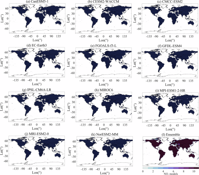
Land mask of PDSI_CMIP6 for each selected climate models and their ensemble mean. Ensemble results (l) show the number of the models with available PDSI estimates.
Validation and application of PDSI_CMIP6
PDSI_CMIP6 was validated against soil moisture simulations using Pearson correlation and linear regression analysis to assess its internal consistency with hydrological components within CMIP6 Earth System Models—relationships not captured in traditional offline PDSI estimates39. To guide potential users, we also provide illustrative examples demonstrating practical applications of PDSI_CMIP6. Temporal changes in PDSI_CMIP6 across different continents and globally were investigated using the area-weighted method to extract data from the gridded product (see Figure S1 for geographical classification)40. Long-term linear trend was estimated using the least square method41 and spatial distribution was presented as the ensemble mean of PDSI_CMIP6. All calculations were performed using the Climate Data Toolbox for MATLAB42. Note the spatiotemporal analysis was illustrated based on the SSP5-8.5 scenario, with results for other scenarios discussed in the supplementary file.