An advanced denoising methodology for Martian surface mineral exploration

Notations

The concepts introduced in this subsection are initially presented. Vectors are represented by lowercase bold letters (e.g., x), where \({\bf{x}}\in {{\mathbb{R}}}^{n}\) indicates a vector of dimension \(n\). Matrices are denoted by bold capital letters (e.g., \({\bf{X}}\in {{\mathbb{R}}}^{{I}_{1}\times {I}_{2}}\)) and represent two-dimensional arrays. Tensors are indicated using Euler-script letters; for instance, the notation \({\mathscr{Y}}\in {{\mathbb{R}}}^{{I}_{1}\times {I}_{2}\times {I}_{3}}\) denotes a third-order tensor with three dimensions.

Image degradation model

The observed CRISM hyperspectral image cube can be expressed as a third-order tensor \({\mathscr{Y}}\in {{\mathbb{R}}}^{{n}_{row}\times {n}_{col}\times L}\) with \(N(N={n}_{row}\times {n}_{col})\) pixels, and \(L\) spectral bands. Assuming that noise is additive with a mean of zero, the image degradation model of CRISM hyperspectral data can be written as

where \(\{{\mathscr{X}},{\mathscr{N}}\}\in {{\mathbb{R}}}^{{n}_{row}\times {n}_{col}\times L}\) denote a clean CRISM HSI image and corresponding noise, respectively.

The spectral vectors of a hyperspectral image tend to lie in a low-dimensional subspace because of the strong correlation between spectral bands33,34. The subspace representation theory has been widely used to solve inverse problems in hyperspectral imaging and has shown promising results35,36. Based on the subspace theory, the clean image \({\mathscr{X}}\) can be expressed as follows:

where columns of \({\bf{C}}\in {{\mathbb{R}}}^{L\times p}(p\,\ll \,L)\) hold an orthogonal basis for the spectral subspace, and elements of \({\mathscr{A}}\in {{\mathbb{R}}}^{{n}_{row}\times {n}_{col}\times p}\) are representation coefficients of \({\mathscr{X}}\) with respect to \({\bf{C}}\). Hereafter, mode-3 slices of \({\mathscr{A}}\) are termed eigenimages. Hence, the image degradation model (1) can be rewritten as follows:

E2E for CRISM denoising

The proposed CRISM hyperspectral image denoising farmwork can be divided into three parts, including subspace representation of CRISM data, self-supervised training phase via noisy eigenimages, and inference phase.

Subspace representation of CRISM data

Given the spectral correlation matrix of the observed data, \({{\mathscr{Y}}}_{(3)}{{\mathscr{Y}}}_{(3)}^{T}/N\), the subspace representation is obtained by performing eigen-decomposition, expressed as

and

where \({\bf{U}}\) is an orthogonal matrix. The eigenvalues in the diagonal matrix \({\bf{S}}\) are ordered by decreasing magnitude. The basis matrix \({\bf{C}}\) can be obtained from \({\bf{U}}\) with the first \(p\) columns. In addition, \(N\) is the total number of image pixels. Therefore, given \({\bf{C}}\), the CRISM denoising problem can be reformulated as an eigenimages denoising with the following formula:

where \({f}_{\theta }(\cdot )\) is the E2E-CRISM denoising network introduced in the next section.

Training phase

In this section, a self-supervised training framework with only noisy CRISM eigenimages is introduced. E2E framework for CRISM data brings two benefits as follows:

We generate two sub-images from a single noisy eigenimage via a neighbor column sub-sampler, inspired by the neighbor2neighbor23. This sub-image generation strategy enables us to train a network without clean images.

The first eigenimage is of high quality, which can help guide the feature extraction of other eigenimage bands.

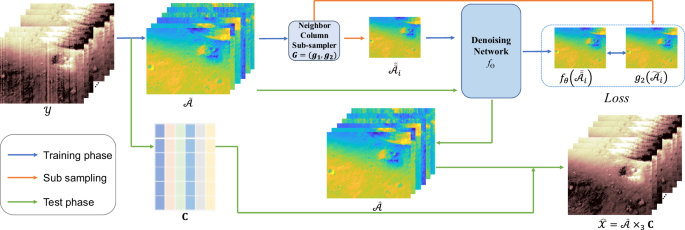
This paper focuses on the utilization of full resolution targeted observations (FRT) image cubes acquired by the \(L\) detector with 231 bands ranging from 1.1127 \(\mu m\) to 2.6285\(\mu m\), among various types of CRISM Mars images. The training of our model utilizes all global CRISM FRT images (a total of 10,406 images, excluding any invalid ones). It is worth mentioning that prior to network training, only photometric angles and atmospheric correction have been rectified using CAT software. The training phase of the E2E-CRISM framework is depicted in Fig. 1 with a blue arrow flow. The modified lightweight RRG network37 is employed as the underlying architecture of our denoising framework, comprising a total of 7 layers. More specifically, the RRG network comprises 2 RRG modules, and each RRG module contains 4 dual attention blocks that utilize channel attention and spatial attention mechanisms. Accordingly, the number of kernels and their size were set to 64 and 3, respectively.

To measure the eigenimage denoising performance, several cost functions have been investigated in the image denoising field, such as \({l}_{1}\) loss, \({l}_{2}\) loss, etc. We adopt \({l}_{1}\) loss to measure the reconstruction accuracy, and TV loss to impose spatial smoothness. Let \(\tilde{{\mathscr{A}}}={\mathscr{Y}}{\times }_{3}{{\bf{C}}}^{T}\) represents noisy eigenimage, hence the total loss function can be expressed as follows:

where \({f}_{\theta }\) is a network parameterized by \(\theta\), and the modified lightweight RRG network31 is adopted in E2E framework. For simplify, let \(\tilde{{{\mathscr{A}}}_{i}}=\tilde{{\mathscr{A}}}(:,:,i)\), \({\tilde{\tilde{{\mathscr{A}}}}}_{i}=cat({g}_{1}(\tilde{{\mathscr{A}}}(:,:,1)),{g}_{1}(\tilde{{\mathscr{A}}}(:,:,i))\), and \({\overline{{\mathscr{A}}}}_{i}=cat(\tilde{{\mathscr{A}}}(:,:,1),\tilde{{\mathscr{A}}}(:,:,i))\). The function of \(cat({\bf{A}},{\bf{B}})\) defines the concatenation of matrix \({\bf{A}}\) and \({\bf{B}}\) along the frequency dimension, and \(\tilde{{\mathscr{A}}}(:,:,1)\) is the first noisy eigenimage with high quality, which is used as a guide image to guide the rest of eigenimages. The \(\alpha\), and \(\gamma\) are two hyperparameters for network training. In addition, \({ {\mathcal L} }_{TV}\) is the TV loss, which can be expressed as follows:

where \({\nabla }_{h}\) and \({\nabla }_{v}\) are the horizontal and vertical gradients of the image \({f}_{\theta }({\tilde{\tilde{{\mathscr{A}}}}}_{i})\), respectively.

Denoising phase

Given that the eigenimage denoising network has been well-trained, the proposed denoising framework contains three steps:

Step 1: Subspace projection of the noisy CRISM HSI \({\mathscr{Y}}\) onto an orthogonal subspace: \({\tilde{{\mathscr{A}}}}_{i}={\mathscr{Y}}{\times }_{3}{{\bf{C}}}^{T}\)

Step 2: Denoise observed eigenimages using the proposed self-supervised network:

where \({f}_{\theta }\) is the well-trained denoising network, and \({\widehat{{\mathscr{A}}}}_{i}\) is the \(i\) th denoised eigenimage.

Step 3: The denoised CRISM HSI data can be multiplied by the estimated eigenimage \(\widehat{{\mathscr{A}}}\) and the spectral subspace bias \({\bf{C}}\), i.e., \(\widehat{{\mathscr{X}}}=\widehat{{\mathscr{A}}}{\times }_{3}{\bf{C}}.\)