This study focuses on the Zhengzhou city cluster as the core research area, as shown in Fig. 1. This region is located in the middle and lower reaches of the Yellow River in China, serving as the heartland of the Central Plains Economic Zone and bearing the dual national strategic tasks of “The Rise of Central China” and “ecological protection of the Yellow River Basin.” The Zhengzhou city cluster is not only the economic center of Henan Province, with a GDP exceeding 4 trillion yuan in 2022, accounting for 45% of the province’s total, but also an important grain production base and emerging manufacturing hub nationwide. The per capita water resource availability is less than 300 cubic meters, just one-seventh of the national average, making it a severely water-scarce area. Agricultural water use accounts for as high as 62% (data from 2023), yet the GDP output per unit of water resources is only one-third that of the Yangtze River Delta, indicating low resource allocation efficiency. Long-term over-extraction of groundwater and rapid industrialization have led to prominent contradictions between water resource carrying capacity and the ecological environment. As the core of the Central Plains Economic Zone, the Zhengzhou city cluster holds significant strategic importance in regional development. Agriculture and manufacturing coexist, leading to high water demand, but utilization efficiency needs improvement. The characteristics of high population density, moderate income levels, and rapid industrialization make it a typical representative of water resource management issues in most developing regions globally. The uniqueness of the Zhengzhou city cluster lies in its “high population density-moderate income level-rapid industrialization” development model, which differs from both the governance paths of developed countries relying on technology or international cooperation and those of China’s coastal developed city clusters. Studying the coupling relationship between water resource carrying capacity, ecological environment, and economic development in this region can provide scientific evidence and practical solutions for sustainable development in similar developing areas.
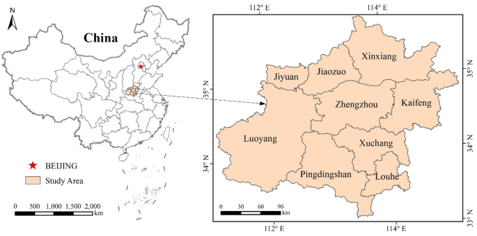
Geographical location map of Zhengzhou city cluster(Produced by ArcMap 10.8).
Research hypothesis
Based on the regional characteristics of the study area and existing theories (growth pole theory, policy intervention theory, system synergy theory), this research proposes three research hypotheses, each supported by practical foundations and logical reasoning: Hypothesis 1: The coupling coordination degree of the WES system in Zhengzhou City Cluster has significantly improved over time, but shows “core-periphery” regional disparities.
Practical Foundation: From 2012 to 2021, Zhengzhou City Cluster underwent policy interventions such as the “Zhongyuan City Cluster Development Plan” (2016) and the “Yellow River Basin Ecological Protection and High-Quality Development Strategy” (2019). The core city Zhengzhou achieved an average annual GDP growth rate of 8.5%, reduced water consumption per 10,000 yuan of GDP from 150 m³ to 100 m³, and improved its ecological environment quality index from 0.65 to 0.82, indicating initial emergence of system synergy effects. However, peripheral cities faced dual pressures from economic transformation and ecological restoration, resulting in a coupling coordination degree 0.15–0.2 units lower than Zhengzhou in 2021, demonstrating significant regional disparities.
Theoretical Support: According to growth pole theory, core cities (Zhengzhou and Luoyang) attract resources through agglomeration effects, achieving initial synergy in the WES system. Peripheral cities lag behind due to insufficient factor supply, leading to regional disparities. However, as policy dividends spread, these disparities will gradually narrow, with overall coupling coordination degree showing an upward trend.
Hypothesis 2 Water scarcity serves as the primary constraint on the coupling coordination of the WES system in Zhengzhou Urban Agglomeration, with its inhibitory effect showing a “first-strong, then weak” trend over time.
Real-world evidence: From 2012 to 2015, water consumption per 10,000 yuan of GDP in Zhengzhou reached 140–150 m³, while per capita water usage was 250–260 cubic meters, indicating low water resource utilization efficiency that became the foremost obstacle to system coordination. After 2016, with the implementation of the “strictest water resource management system”, water consumption per 10,000 yuan of GDP dropped to 100 m³, reducing water resource barriers by 15–20%. However, this improvement still exceeded the reduction rates in ecological environment (30% decrease) and socio-economic factors (25% decrease), remaining a core constraint.
Theoretical support: According to resource constraint theory, during the initial stage of regional development, water scarcity as a fundamental resource directly restricts economic growth and ecological conservation, becoming the “weak link” in system coordination. With the promotion of water-saving technologies and optimized management leading to improved water utilization efficiency, its constraining effect gradually diminishes. However, since the region’s per capita water resources remain below the “extreme water scarcity” threshold of 300 m³, water resources will continue to be the primary constraint in the long term.
Hypothesis 3 Implementing differentiated regulatory measures tailored to the unique characteristics of urban systems can significantly enhance the coupling coordination of the WES system.
Real-world context: The Zhengzhou city cluster exhibits pronounced systemic differentiation ——Zhengzhou and Luoyang face acute ecological pressures conflicting with socioeconomic development, while Pingdingshan and Jiaozuo confront urgent water resource constraints requiring ecological restoration. Xuchang and Kaifeng demonstrate insufficient synergy between socioeconomic upgrading and water resource efficiency, making single-regulation approaches inadequate for all cities.
Theoretical foundation: According to system synergy theory, coordinated development of the WES system requires a “weakness-filling” approach. Designing targeted regulatory measures for each city’s core challenges enables precise optimization, thereby improving overall coupling coordination. Policy intervention theory further indicates that differentiated policies mitigate efficiency losses from blanket measures, enhancing the feasibility and effectiveness of regulatory solutions.
Indicator system
WES is a complex coupled system involving multiple dimensions, including water resources, ecological environment, and socio-economic factors (Fig. 2). To uncover the interaction mechanisms among these elements, this study developed a comprehensive evaluation index system covering three dimensions: water resources, socio-economic systems, and ecological environment systems.
WES system multidimensional coupling relationship and mechanism illustration
The three subsystems of WES system have a “two-way feedback-hierarchical nesting” structure. The core functions, key elements and interaction paths of each subsystem are as follows:
1.
Core subsystem functional positioning
Water Resources System (Foundational Support): Serving as both the “lifeline” of ecological environment and the “constraint line” for socio-economic development, it performs three core functions: supply, regulation, and purification. Key elements include supply-related indicators such as total water resources (A10) and annual precipitation (A11), efficiency-related indicators like water consumption per 10,000 yuan GDP (A15) and per capita water usage (A14), as well as allocation-related indicators such as total water supply (A13) and ecological water ratio (A20). These directly determine the carrying capacity of the ecological environment and the scale of socio-economic development.
Ecological Environment System (Intermediate Buffer): Acting as a “bridge” connecting water resources with socio-economy, it fulfills roles in purification, regulation, and support. Core elements include pollution control indicators like centralized urban sewage treatment rate (A17) and industrial wastewater discharge volume (A22), ecological restoration indicators such as green coverage rate in built-up areas (A18) and ecological water ratio (A20), along with environmental pressure indicators including industrial sulfur dioxide emissions (A23) and industrial smoke/dust emissions (A24). The quality of these indicators directly impacts water resource circulation efficiency and socio-economic sustainability.
Socioeconomic System (Superior Driving Force): As the “driving force” of system development, it influences water resources and ecological environment through the “demand-technology-policy” chain. Core elements include economic scale indicators such as GDP total (A3) and per capita disposable income (A6), industrial structure indicators like the ratio of primary/secondary/tertiary industries (A1/A2/A9), and water consumption structure indicators including agricultural/industrial/lifestyle water usage ratios (A4/A5/A8). The development model directly determines water consumption intensity and ecological pressure.
2.
Multi-dimensional coupling pathways between subsystems
Positive Synergy Pathways: ① Water Resource System → Ecological Environment System: Increased ecological water use ratio (A20) promotes higher green coverage in built-up areas (A18), enhancing the ecosystem’s water conservation capacity; ② Ecological Environment System → Socioeconomic System: Improved centralized urban sewage treatment rate (A17) reduces industrial wastewater pollution, ensures agricultural and industrial water safety, and indirectly drives GDP growth (A3); ③ Socioeconomic System → Water Resource System: Higher tertiary industry proportion (A9) decreases industrial water consumption (A5), lowers water usage per 10,000 yuan of GDP (A15), and improves water resource efficiency.
Negative Constraints Pathways: ① Water Resource System → Socioeconomic System: Insufficient total water resources (A10) restrict agricultural irrigation and industrial production, slowing growth in primary/secondary industries (A1/A2); ② Socioeconomic System → Ecological Environment System: Excessive secondary industry proportion (A2) increases industrial wastewater discharge (A22) and sulfur dioxide emissions (A23), exacerbating environmental pollution; ③ Ecological Environment System → Water Resource System: Excessive industrial wastewater discharge (A22) contaminates surface and groundwater sources, reduces available water resources (A10), creating a vicious cycle of “pollution-water scarcity-development constraints”.
3.
System-wide regulation logic
The WES system achieves coordinated coupling through a hierarchical linkage of “Objective Layer-Criterion Layer-Indicator Layer”: The Objective Layer focuses on synergistic coordination among “water resource efficiency, ecological environment improvement, and socio-economic growth”; the Criterion Layer connects objectives with indicators through three dimensions: water utilization efficiency, ecological pressure, and socio-economic development; while the Indicator Layer quantifies subsystem status using 24 specific metrics.
Design principles and details of the index systemCriteria for inclusion/exclusion of indicators
(1)
Scientificity and representativeness: Indicators should be able to objectively reflect the core characteristics of the WES system. For example, total water resources (A10) directly represent regional water resources endowment, and water consumption per 10,000 yuan of GDP (A15) reflects water resource utilization efficiency.
(2)
Policy relevance: Indicators directly related to the “four waters and four determinations” principle of the Yellow River Basin and the national sustainable development strategy are given priority, such as ecological water use ratio (A20) and industrial wastewater discharge (A22).
(3)
Data availability and continuity: All index data are from authoritative statistical yearbooks (2012–2021) to ensure the integrity of the time series. For example, detailed water quality indicators (such as heavy metal concentration) are not included due to missing data in some years.
(4)
System interactivity: Indicators should be able to capture the dynamic feedback between subsystems. For example, the proportion of industrial water use (A5) is not only affected by economic structure but also reacts to water resource pressure.
Description of potential missing indicators
(1)
Climate resilience indicators (such as the frequency of extreme precipitation): Due to the insufficient spatial resolution of regional scale meteorological data and redundancy with existing indicators (annual precipitation A11, water yield coefficient A12), they are not included separately.
(2)
Water quality detail indicators (such as COD, ammonia nitrogen concentration): although important, they are limited by the continuity of data in some cities, so the comprehensive index “industrial wastewater discharge (A22)” is used instead.
(3)
Social equity indicators (such as the Gini coefficient of water resources allocation) are not included due to the controversial quantitative methods, but are indirectly reflected through “per capita water consumption (A14)”.
Dynamic feedback and nonlinear relationship capture
(1)
Direct interaction indicators:
A.
Negative “economic-environmental” feedback chain is formed between the proportion of industrial water (A5) and the discharge of industrial wastewater (A22).
B.
The proportion of ecological water (A20) and the green coverage rate of built-up areas (A18) reflects the positive synergistic effect between “water resources and ecology”.
(2)
Nonlinear representation:
A.
Coupling coordination degree model (Formula 15–16) is used to quantify the nonlinear threshold effect between subsystems, such as the coordination degree decreases when economic growth exceeds water resource carrying capacity.
B.
Improve the LSTM model (Sect. 2.3.5) by embedding industry proportion constraints (A1 + A2 + A9 = 100%), forcing the dynamic balance relationship between learning indicators.
The 24 indicators in Table 1 have been validated through sensitivity analysis for their necessity. Removing any of these indicators would result in a decrease in the explanatory power of the coupling coordination degree model by more than 5% (based on the R²test). Future research could incorporate higher-resolution data to enhance climate resilience metrics, but the current system is already capable of effectively supporting the comprehensive evaluation needs of the WES system.
Research methodCalculation of indicator weights
The data in this paper mainly comes from the “Henan Province Water Resources Bulletin,” “Henan Province Statistical Yearbook,” “China City Statistical Yearbook,” and “Henan Province Environmental Statistical Annual Report” for the period 2012–2021, as well as the “Water Resources Bulletin,” “Statistical Yearbook,” and “National Economic and Social Development Statistical Bulletin” of various prefecture-level cities in the study area. Missing data in the yearbooks were filled using linear interpolation.
First of all, the index is standardized. The core innovation lies in the game theory combination weighting method, which is as follows:
1.
Basic empowerment method selection logic
Entropy method and CRITIC method are selected as the basic methods, both of which are objective weighting methods to avoid subjective bias, but a single method has limitations —— entropy method ignores the independence between indicators, CRITIC method weakens the difference of data distribution.
2.
Game theory combinatorial weighting improvement.
Weight fusion is realized through the following steps to solve the defects of a single method: (1) Calculate the entropy method weight vector \(\:{\text{W}}_{1}\) and the CRITIC method weight vector \(\:{\text{W}}_{2}\) separately. (2) Let the combination coefficients \(\:{a}_{1}\) and \(\:{a}_{2}\) (\(\:{a}_{1}\)+\(\:{a}_{2}\)=1) to construct the combined weights W=\(\:{a}_{1}{\text{W}}_{1}\)+\(\:{a}_{2}{\text{W}}_{2}\). (3) Aim for “minimizing weight deviation,” solve the optimal combination coefficients through matrix differentiation, ensuring that the final weights reflect data dispersion while maintaining indicator independence.
Experimental results show that this method improves the R² of WES system evaluation results by 8%−10%, which is better than the single weighting method (the weight calculation results are shown in Table 2).
Comprehensive development level of the WES system
In this paper, the comprehensive index method is used to evaluate and analyze the three subsystems of the WES system and the comprehensive development level of the WES system23. The calculation formula is as follows:
$$U = \mathop \sum \limits_{j = 1}^m {W_j}x_{ij}^*$$
(1)
$$T = {\beta _1}{U_1} + {\beta _2}{U_2} + {\beta _3}{U_3}$$
(2)
Where: U represents the overall development level of subsystems;\(\:{\text{U}}_{1}\), \(\:{\text{U}}_{2}\), and \(\:{\text{U}}_{3}\)represent the overall development levels of the socio-economic, water resources, and ecological environment subsystems, respectively; T represents the overall development level of the WES system; \(\:{{\upbeta\:}}_{1}\), \(\:{{\upbeta\:}}_{2}\), and \(\:{{\upbeta\:}}_{3}\) represent the importance levels of the urbanization, water resources, and ecological environment subsystems, respectively. This study considers all three subsystems to be equally important, so \(\:{{\upbeta\:}}_{1}={{\upbeta\:}}_{2}={{\upbeta\:}}_{3}=1/3\).
WES system coupling and coordination evaluation model
The Coupling Coordination Degree Model quantitatively evaluates two fundamental concepts: coupling degree and coupling coordination degree24. The coupling degree is a physical concept that indicates the extent of mutual influence between different modules, involving dependencies such as call relationships, control relationships, and data transfer relationships. Essentially, it measures the degree of interconnection and interaction among two or more entities or systems25. The coupling coordination degree evolved from the coupling degree, primarily reflecting the overall effect and synergy of interactions between multiple modules from an integrated perspective. It overcomes the illusion of high-level coupling at low levels and further characterizes whether the effects of interactions between modules are mutually reinforcing at high levels or mutually restrictive at low levels26.
This paper mainly discusses the degree of interaction, influence, dependence, and coordination among WES systems in Zhengzhou urban agglomeration, to measure the coupling and coordinated development status of these three subsystems. The calculation formula is as follows:
$$C = {\left[ {\frac{{{U_1} \times {U_2} \times {U_3}}}{{{{\left( {\frac{{{U_1} + {U_2} + {U_3}}}{3}} \right)}^3}}}} \right]^{1/3}}$$
(3)
$$D = \sqrt {C \times T}$$
(4)
Where: C is the coupling degree and takes the value of [0,1]; D is the coupling coordination degree and takes the value of [0,1].
This paper divides the coupling coordination degree into levels based on existing research, as shown in Table 3.
WES system barrier identification
To identify the impact and constraining factors of various evaluation indicators on the coupling coordination degree of the WSE composite system in the Zhengzhou city cluster, an obstacle analysis model was used to measure and diagnose the obstacle factors affecting the coupling coordination degree of the two systems27. The concepts of “indicator contribution, “indicator deviation,” and “obstacle degree” were introduced. A smaller obstacle degree indicates that the indicator has a lesser hindrance to coordination. The specific calculation formula is as follows:
$${v_j} = 1 – r_{ij}^*$$
(5)
$${M_j} = \frac{{\omega _{ij}^*{v_j}}}{{\mathop \sum \nolimits_{j = i}^m {\omega _{ij}}{v_j}}}$$
(6)
Where: \(\:{\text{M}}_{\text{j}}\) is the degree of obstacle; \(\:{{\upomega\:}}_{\text{i}\text{j}}^{\text{*}}\) is the weight of the jth index, that is, the contribution of the index; \(\:{\text{r}}_{\text{i}\text{j}}^{\text{*}}\) is the standardized data of the jth index in the i year; \(\:{\text{v}}_{\text{j}}\) is the deviation of the index; m is the number of indexes.
Improve the LSTM model
LSTM is a special type of recurrent neural network structure, commonly used for processing and learning time series data. At its core are internal “memory cells” and a series of “gate” mechanisms. These gates control the flow of information in and out, helping the model selectively retain or forget information28. A typical LSTM unit includes several key steps: First, it constructs a cell state similar to a “belt,” which can traverse the entire sequence through minimal linear operations and passes, allowing information to propagate over long periods within the sequence. Then, through the forget gate, it performs a linear transformation on the input (including the previous year’s prediction) and the hidden state, filtering out the most valuable information for future predictions while discarding less important historical data.
$${f_t} = \sigma \left( {{W_f}\left[ {{h_{t – 1}},{a_t} + {b_f}} \right]} \right)$$
(7)
Where: \(\:{\upsigma\:}\)is the sigmoid function, \(\:{\text{W}}_{\text{f}}\) is the weight matrix, \(\:{\text{h}}_{\text{t}-1}\)is the internal state information retained by the model in the previous time step, \(\:{\text{a}}_{\text{t}}\)is the input data received in the current time step, and \(\:{\text{b}}_{\text{f}}\) is the bias term.
It then determines how much new information will be added to the cell state at the current time step by inputting the gate. It helps the model effectively update the cell state in the training data from 2012 to 2019 to generate the basis for future predictions.
$${i_t} = \sigma \left( {{W_i}\left[ {{h_{t – 1}},{a_t} + {b_i}} \right]} \right)$$
(8)
$$C_{k}^{‘} = \tanh (W_{c} \cdot \left[ {h_{{t – 1}} ,a_{t} + b_{i} } \right])$$
(9)
Where: \(\:{C}_{k}^{{\prime\:}}\)‘is the candidate value used to generate new information; tanh is the hyperbolic tangent function.
Finally, the output gate determines how much information in the hidden state (also the output of the LSTM unit) at the current time step will be used to predict the indicator value for the next year, while providing key input for the prediction of subsequent time steps, ensuring that the model can extrapolate future trends from the historical data of 2012–2019 to the future trends of 2020–2026.9
$$O_{t} = \sigma \left( {W_{o} \cdot \left[ {h_{{t – 1}} ,a_{t} + b_{o} } \right]} \right)$$
(10)
$$h_{t} = O_{t} \cdot \tanh \left( {C_{k}^{‘} } \right)$$
(11)
Where: \(\:{O}_{t}\)is the output vector of the output gate, which determines how much information from the current cell state will be passed through the output gate to the hidden state; \(\:{h}_{t}\) is the hidden state vector of the current time step, which is also the output of the LSTM unit.
Traditional LSTM models have three major problems in WES system prediction: low accuracy of small samples (time series
1.
Problem 1: The prediction accuracy is insufficient under small sample data: Improved Measures —— Multi-dimensional Feature Cross-Input: Traditional LSTM models only input single subsystem indicators. This study integrates water resources, ecological environment, and socio-economic indicators through cross-combination inputs. For instance, indicators with interactive relationships such as “industrial water consumption ratio -industrial wastewater discharge ” and “ecological water proportion -built-up area green coverage rate ” are input in pairs. This enhances the model’s ability to extract multi-system collaborative features.
2.
Problem 2: Predictions violate physical reality: (1) Training Phase: Adjust the loss function by incorporating a constraint loss term\(\:\:\:{\text{L}}_{\text{c}\text{o}\text{n}\text{s}\text{t}\text{r}\text{a}\text{i}\text{n}\text{t}}\), defined as \(\:{\text{L}}_{\text{t}\text{o}\text{t}\text{a}\text{l}}={\text{L}}_{\text{M}\text{S}\text{E}}+{\uplambda\:}{\text{L}}_{\text{c}\text{o}\text{n}\text{s}\text{t}\text{r}\text{a}\text{i}\text{n}\text{t}}\) (Where \(\:{\text{L}}_{\text{M}\text{S}\text{E}}\) represents root mean square error, \(\:{\uplambda\:}\)is the constraint weight set to 0.3). The constraint loss term is calculated as \(\:{\text{L}}_{\text{c}\text{o}\text{n}\text{s}\text{t}\text{r}\text{a}\text{i}\text{n}\text{t}}\)=\(\:\left|(\text{A}4+\text{A}5+\text{A}8+\text{A}20)\right|-100+\left|\left(\text{A}1+\:\text{A}2+\:\text{A}9\right)\right|-100\), ensuring the model maintains balance between “total water usage ratio = 100%” and “total industrial proportion = 100%”.