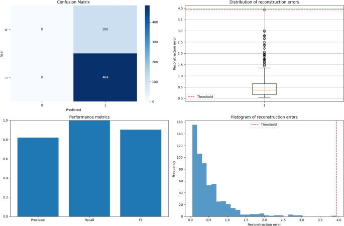
In this work, we employ several machine learning concepts that we define here for clarity. Classes refer to the categories into which we organize sounds – in our case, Schafer’s three categories: keynotes, sound signals, and soundmarks. Each audio sample is assigned to one of these classes based on its characteristics. Intra-class distance measures how similar sounds are within the same category – for example, how similar different keynote sounds are to each other. A smaller intra-class distance indicates that sounds in that category share more common features, making them easier to identify as a group. The reconstruction error represents the difference between an original audio signal and its reconstructed version after compression by the VAE. When the VAE processes an audio file, it first compresses it into a simplified representation (encoding), then attempts to recreate the original from this compression (decoding). The reconstruction error measures how much information was lost in this process – unusual or distinctive sounds typically have higher reconstruction errors because they are harder for the model to compress and recreate accurately. To ensure accessibility for readers from diverse backgrounds, Fig. 4 provides definitions of additional key technical terms used throughout this work.
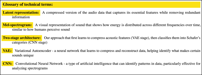
Key technical terms used in this work..
This two-stage architecture was specifically chosen to operationalize Schafer’s theoretical framework computationally. The VAE enables unsupervised discovery of acoustic patterns without labeled data, learning what makes sounds distinctive – crucial given the subjective nature of soundscape perception. The CNN then maps these learned features to Schafer’s categories, benefiting from pre-extracted relevant patterns rather than raw spectrograms. This separation provides interpretability through reconstruction error as a novel distinctiveness metric. We selected PyTorch for reproducibility, mel-spectrograms for their perceptual relevance matching human auditory processing, and Head Acoustics binaural recording to capture spatial characteristics essential to soundscape perception. The 70th/30th percentile thresholds were empirically determined from energy distributions, aligning with psychoacoustic principles of auditory stream segregation where sounds emerging 6-10 dB above background become perceptually distinct.
Note that while soundscape studies typically employ continuous metrics (LAeq, loudness, roughness), our approach necessarily discretizes sounds into Schafer’s three categories. This discretization parallels established practices like categorizing noise levels (quiet/moderate/loud) or the ISO 12913-3 quadrants (pleasant/unpleasant \(\times\) eventful/uneventful), making complex acoustic environments interpretable for preservation decisions.
System architecture overview
The audio classification system operates as a two-stage pipeline, as illustrated in Fig. 5. The first stage utilizes a Variational Autoencoder (VAE)45,46 for feature learning and dimensionality reduction of audio data. The second stage employs a Convolutional Neural Network (CNN) classifier47 that categorizes sounds according to Schafer’s taxonomy based on the features extracted by the VAE.
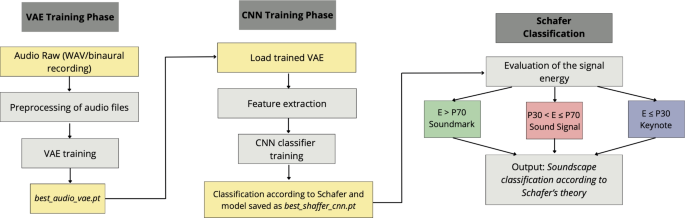
Overview of the two-stage audio classification system based on VAE and CNN.
This architecture leverages the strengths of both models: the VAE’s ability to learn compact, informative representations and the CNN’s discriminative power for classification tasks.
Audio Preprocessing
All audio samples in the experiments are preprocessed using a consistent pipeline to ensure standardized inputs to the neural networks. The preprocessing is implemented using the AudioPreprocessor class48:
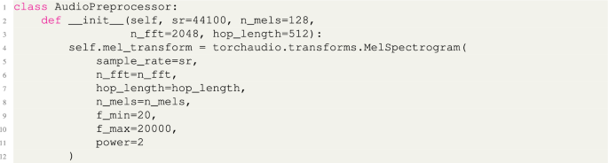
Audio preprocessor implementation.
The key preprocessing parameters are shown in Table 3.
This preprocessing stage converts raw audio waveforms into mel-spectrograms, which capture the frequency content of audio signals in a way that approximates human auditory perception. The mel-spectrogram representation is particularly suitable for audio classification tasks as it emphasizes perceptually relevant frequency bands. The study conducts spectral analysis of binaural audio recordings from the Pescara University District using mel-scale frequency analysis, which provides a perceptually-relevant representation by mimicking human auditory perception. The researchers compute mel spectrograms using a 2048-point FFT with 512-sample hop length, generating 128 mel frequency bins that capture spectral evolution over time. Through a Variational Autoencoder (VAE) architecture, the analysis examines reconstruction error of these spectral representations to distinguish between different acoustic conditions in the university district environment. The VAE learns to encode complex spectral patterns present in binaural recordings into a lower-dimensional latent space and reconstruct them, with reconstruction error serving as a discriminative feature for audio classification. This spectral-based methodology enables effective characterization of the acoustic environment by focusing on frequency domain properties and their temporal variations.
The Fig. 6 illustrates how the Variational Autoencoder processes binaural audio recordings from the Pescara University District, comparing original mel-spectrograms with their reconstructions.
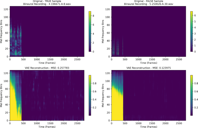
Original mel-spectrograms (top) and VAE reconstructions (bottom) for TRUE and FALSE samples from Pescara University District binaural recordings. Reconstruction errors (MSE: 0.257783 vs 0.123975) demonstrate the VAE’s discriminative capability for acoustic classification.
The Fig. 6 presents two contrasting examples: a TRUE sample (4-196671-A-8.wav) and a FALSE sample (5-250026-A-30.wav), each showing distinct acoustic characteristics. The original spectrograms reveal different temporal and spectral patterns between the two samples. The TRUE sample exhibits concentrated energy in lower frequency bins during the initial time frames, while the FALSE sample shows a more distributed frequency response with activity across multiple mel frequency bins. The VAE reconstructions demonstrate the model’s ability to capture essential spectral features while introducing reconstruction errors that serve as discriminative indicators. The TRUE sample achieves a higher reconstruction error (MSE: 0.257783) compared to the FALSE sample (MSE: 0.123975), suggesting that the reconstruction error effectively differentiates between acoustic conditions. The reconstructed spectrograms show how the VAE learns to encode and decode the complex spectral patterns, with the yellow-green regions indicating higher energy reconstruction in the lower frequency bands. The reconstruction quality varies between samples, with the error magnitude serving as a classification feature for distinguishing different acoustic environments within the university district.
Variational autoencoder architecture
The VAE consists of an encoder network that maps the input mel-spectrogram to a latent space distribution, and a decoder network that reconstructs the mel-spectrogram from samples drawn from this distribution49.
The VAE was trained with the parameters shown in Table 4.
The Adam optimizer50 was used the VAE with an adaptive learning rate schedule. For the VAE, the learning rate was started at 1e-4 and reduced by a factor of 10 at epochs 100 and 150.
The VAE compresses mel-spectrograms from 128\(\times\)2756 dimensions (approximately 353,000 values) to a 256-dimensional latent vector, achieving a 1,400\(\times\) compression ratio. This “meaningful representation” preserves perceptually relevant features (temporal patterns, spectral envelopes, harmonic structures) while discarding redundancy. The reconstruction error serves as a distinctiveness metric: keynotes (common sounds) have low reconstruction error, sound signals moderate error, and soundmarks (unique sounds) high error. This compressed representation provides the CNN with pre-extracted relevant features rather than raw spectrograms, improving classification efficiency and accuracy.
The model processes acoustic features as follows: mel-spectrograms provide time-frequency representations analogous to psychoacoustic analysis; the VAE compresses these into latent features similar to principal components in soundscape studies; reconstruction error serves as an acoustic distinctiveness metric; the CNN maps these features to Schafer’s categories based on learned patterns corresponding to L90-like levels for keynotes, L10-like peaks for sound signals, and unique spectral signatures for soundmarks.
Encoder
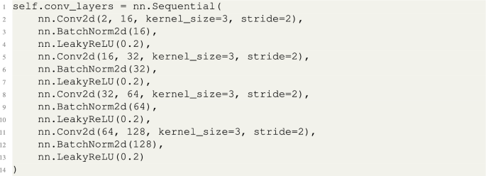
The encoder architecture is implemented as follows:
The encoder outputs parameters for a multivariate Gaussian distribution in the latent space51: mean (\(\mu\)) and log-variance (\(\log \sigma ^2\)). This distribution is represented mathematically as:
$$\begin{aligned} q_\phi (z|x) = \mathcal {N}(\mu _\phi (x), \sigma ^2_\phi (x)) \end{aligned}$$
(1)
where \(\phi\) represents the encoder parameters, x is the input mel-spectrogram, and z is the latent variable.
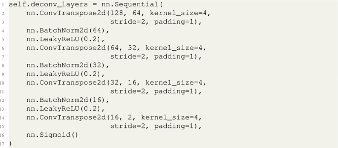
Decoder
The decoder architecture is implemented symmetrically:
The decoder implements the probability distribution:
$$\begin{aligned} p_\theta (x|z) = f_\theta (z) \end{aligned}$$
(2)
where \(\theta\) represents the decoder parameters and \(f_\theta\) is the function implemented by the decoder network.
VAE loss function
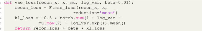
The VAE is trained to minimize the combined reconstruction loss and Kullback-Leibler divergence:
$$\begin{aligned} \mathcal {L}(\theta , \phi ; x) = \mathbb {E}_{q_\phi (z|x)}[\log p_\theta (x|z)] – \beta DKL(q_\phi (z|x)||p(z)) \end{aligned}$$
(3)
where \(\beta\) is a hyperparameter controlling the weight of the KL term. This is implemented as:
CNN classifier architecture
After training the VAE, we use the encoder to extract features from audio samples. These features are then passed to a CNN classifier for categorization according to Schafer’s taxonomy.
The CNN implements four convolutional blocks, each followed by batch normalization. The convolutional operation is defined as:
$$\begin{aligned} Conv(X)_{i,j} = \sum _{m,n} K_{m,n} \cdot X_{i+m,j+n} + b \end{aligned}$$
(4)
The batch normalization operation is defined as:
$$\begin{aligned} BN(x) = \gamma \cdot \frac{x – \mu _B}{\sqrt{\sigma ^2_B + \epsilon }} + \beta \end{aligned}$$
(5)
where \(\mu _B\) is the batch mean, \(\sigma ^2_B\) is the batch variance, \(\gamma\) and \(\beta\) are learned parameters, and \(\epsilon\) is a small constant for numerical stability.
Classification based on Schafer’s Theory
The final layer of our CNN outputs probabilities for each of Schafer’s categories. To align with Schafer’s theoretical framework, we calculate the energy of the signal and apply thresholds based on percentiles:
$$\begin{aligned} E = \frac{1}{N}\sum _{i=1}^{N}|x_i| \end{aligned}$$
(6)
The classification is then determined as:
$$\begin{aligned} {\left\{ \begin{array}{ll} E > P_{70} & \text {Soundmark} \\ E \le P_{30} & \text {Keynote} \\ P_{30}
(7)
where \(P_{70}\) and \(P_{30}\) represent the 70th and 30th percentiles of energy across the dataset.
This is implemented as:
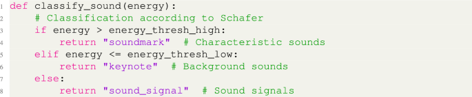
Sound classification according to Schafer.
Data acquisition in situ
It was conducted a real-world case study using binaural monitoring of the university district in Pescara, Italy, to create an authentic neighborhood dataset. We applied the two-stage neural network architecture system to analyze the binaural recordings from the university campus. Located on the Adriatic coast of central Italy, Pescara is a vibrant city with approximately 120,000 inhabitants. The university district is situated in the southern part of the city, where the campus of “G. d’Annunzio” University creates a distinctive urban environment characterized by a mix of academic buildings, student gathering spaces, and surrounding residential and commercial areas. Figure 7 illustrates the study area.
The university district was selected as validation site for several reasons: (1) it provides acoustic diversity with clear examples of all three Schafer categories – keynotes (ventilation systems, ambient movement), sound signals (bells, announcements), and soundmarks (distinctive bell tower, cultural events); (2) it offers a semi-controlled environment with accessible community for validation studies; (3) it enabled systematic temporal sampling across different schedules (lectures/breaks, weekdays/weekends). The site naturally includes many sound categories from the training datasets (air conditioner, car horns, sirens) while also presenting unique sounds not in the training data, testing the model’s ability to generalize to new acoustic environments.
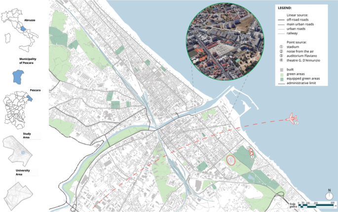
Map of the study area showing the university district of Pescara with the G. d’Annunzio University campus and surrounding urban context. Map created using Adobe Illustrator 2023 (Adobe Inc., https://www.adobe.com/products/illustrator.html) based on AutoCAD base map files.
The acoustic monitoring was conducted over a six-week period using a Head Acoustics GmbH Herzogenrath (Type BSU; S/N 1580028; T/N A01) binaural recording system, which accurately replicates human hearing perception through its anatomically correct ear simulator. As illustrated in Fig. 8, the recording equipment was strategically placed at four different locations across the campus, capturing the soundscape during various time segments (morning, afternoon, evening) and on different days of the week (including weekdays and weekends) to ensure comprehensive temporal coverage of the acoustic environment.
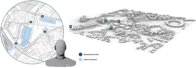
Spatial distribution of acoustic measurement points (dark blue markers) and points of interest (light blue areas) within the university district of Pescara. The figure shows both a detailed 2D map (left) and a 3D representation of the urban context (right), along with the binaural recording system used for data collection. 3D visualization created using Rhinoceros 3D 5.0 (https://www.rhino3d.com/). Map and graphic elements created using Adobe Illustrator 2023 (Adobe Inc., https://www.adobe.com/products/illustrator.html). Binaural head photographs taken by the authors (equipment: BSU head, S/N 15080028).
The prominent characteristics of the university zone include a central pedestrian plaza where students congregate between classes, tree-lined pathways that provide buffer zones between academic buildings, and the intersection of campus life with surrounding urban activities. The area experiences distinct sound patterns influenced by academic schedules, with notable variations between lecture periods and breaks, as well as between term time and holidays.
The dataset comprises 1,410 stereo audio tracks, each with a duration of 10 seconds. All recordings are available in the GitHub repository at https://gitlab.com/sammy-jo/two-stage-architecture-for-soundscape-classification-and-preservation.