Transformer windings defects identification using frequency response analysis and advanced data visualization techniques

The study utilizes a three-phase 1200 kVA power transformer with a voltage rating of 20/0.4 kV (D/Yg connection), representing a typical distribution transformer configuration commonly employed in power systems. The transformer features distinct winding designs for high and low voltage sides to facilitate comprehensive fault analysis. The high-voltage winding comprises 70 interleaved disks with 80 turns per disk (totaling 5600 turns), utilizing round conductors with an inner diameter of 987 mm and outer diameter of 1086 mm. In contrast, the low-voltage winding employs a continuous layer design with 112 turns, featuring round conductors of 823 mm and 891 mm inner and outer diameters respectively. The core structure measures 2033 mm in height and 3785 mm in length, with winding heights of 1154 mm (HV) and 1249 mm (LV). The transformer’s electrical characteristics include a 2.431% impedance at 50 Hz frequency, with Kraft paper and mineral oil serving as the primary insulation materials. To systematically evaluate fault detection capabilities, ten distinct severity levels of three fundamental fault types (axial displacement, radial deformation, and short circuit) were artificially induced at strategic locations across all three phases (A, B, and C). The complete parametric details of these fault configurations are comprehensively documented in Tables 1, 2 and 3 to ensure reproducibility and facilitate comparative analysis.

a) Short Circuit Fault Simulation: This study implemented ten distinct levels of inter-disk short circuit faults at specified disk pairs in the HV winding. The investigated disk pairs included 11–12, 13–15, 18–20, 21–24, 25–26, 27–29, and 32–35, with additional analysis of combined faults at disks 11–12/25–26 and 18–20/27–29. Table 1 shows these simulations:

b) Axial Displacement: Ten progressive levels of axial displacement faults were systematically simulated by displacing the HV winding relative to the LV winding in precise 6.25 mm increments, corresponding to 1–5% of the total winding height (1154 mm). This resulted in displacement magnitudes ranging from 12.5 mm (1.08%) to 62.5 mm (5.41%), covering both minor misalignments and severe deformations observed in practical scenarios. Table 2 shows how these faults created.

c) Radial Deformation: This study systematically investigated radial deformation (RD) by introducing ten distinct fault levels through controlled mechanical deformation of the disk winding. The simulation encompassed various deformation patterns, including single-axis (Fig. 4a), dual-axis opposed (Fig. 4b), three-axis (Fig. 4c), and four-axis symmetric (Fig. 4 d) configurations, with the angular position fixed at θ = 45° for standardization. The deformation severity was precisely quantified using the ratio d/R (Eq. 20), where d represents the radial bending magnitude (d = R – R₁) and R denotes the original average radius. The complete parameter sets for all test cases, including detailed geometric specifications and deformation patterns, are comprehensively documented in Table 3, while Fig. 4 (a)~(d) visually illustrates the various deformation modes.

The power transformer’s dimensions, specifications, and capacity are given in Table 4.

Fig. 4

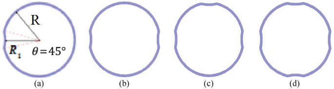
deforming the winding along (a) one axis (b) two axes (c) three axes (d) four axes.

FRA simulation results

The impacts of RD, AD, and SC faults on the transformer’s FRA waveforms are illustrated in Figs. 5(a)–(c) for ten levels of each fault. This study employs an OMICRON analyzer to conduct the FRA measurements. Although the FRA changes are visible in Fig. 5, their analysis is highly challenging. Additionally, low-level fault recognition poses a challenge for conventional FRA. However, the proposed method automates the interpretation process and can be readily applied to FRA, as described below.

Fig. 5

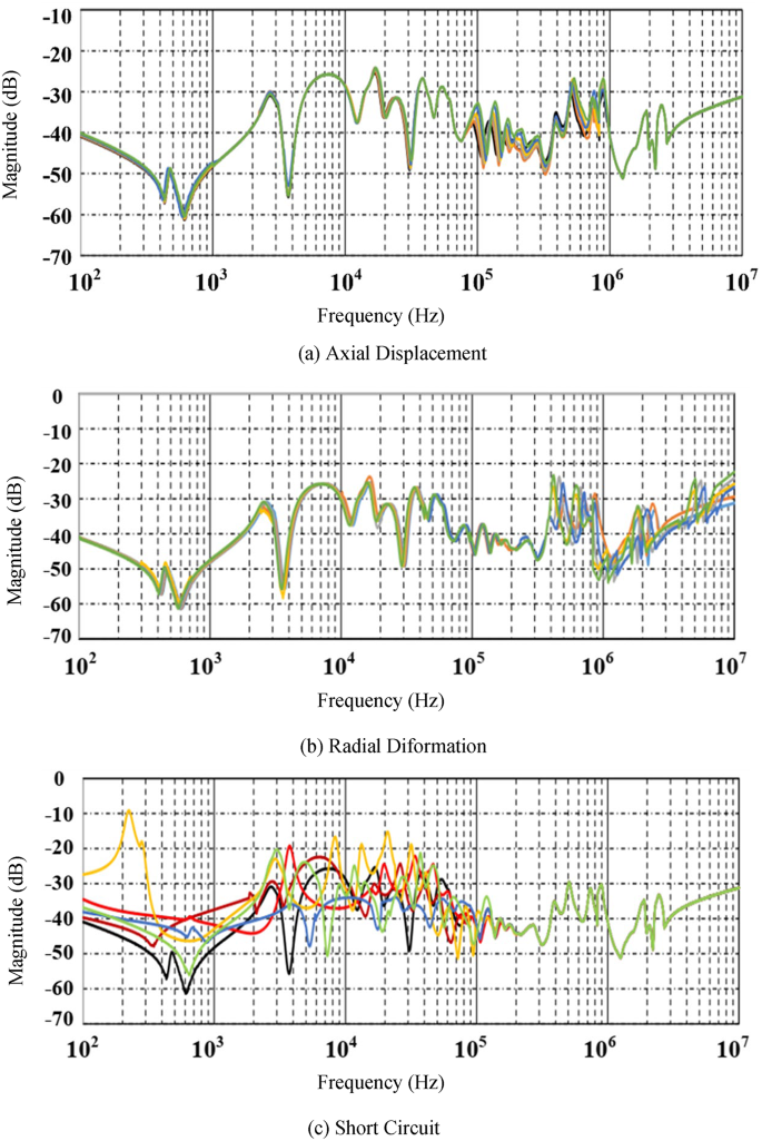
The variation of FRA measurements due to AD, RD, and SC defects in different faults.

Three proposed methods simulations and results

This section reports the results of PCA, FA, and FCA for detecting transformer winding faults. The analysis was performed using R software version 3.6.1 and Minitab version 18. Subsection A presents the PCA results, while Subsections B and C provide the FA and FCA results, respectively.

C.1. Results of PCA to diagnose winding faults

This section presents the results of using PCA for fault detection to diagnose winding faults in the transformer. The eigenvalues of the correlation matrix for variables at low frequency are shown on the left side of Fig. 6a. As shown, only the first two values are greater than 1. The right side of Fig. 6a illustrates that these variables can be classified into two categories: healthy, AD, RD, and SC systems. Consequently, at low frequencies, the RD and AD data are similar to those of a healthy system. However, PCA does not confirm this similarity for SC data. Similarly, the eigenvalues of the mid-frequency correlation matrix are presented on the left side of Fig. 6b, where again only the first two values exceed 1.

Fig. 6

Eigen-values plot for the correlation matrix and the first two loading components for PCA. (a) low-frequency, (b) middle-frequency, (c) high-frequency.

The right side of Fig. 6b shows that these variables can be classified into two categories: healthy, SC, RD, and AD systems. Consequently, at mid-frequency, the SC and RD data show similarity with a healthy system. However, PCA does not confirm this similarity for AD data. The left side of Fig. 6c displays the eigenvalues of the high-frequency correlation matrix variables, where only the first two values exceed 1. The right side of Fig. 6c demonstrates that these variables can again be classified into two categories: healthy, SC, AD, and RD systems. At high frequencies, the SC and AD data are similar to those of a healthy system, while PCA fails to establish this similarity for RD data.

C.2. Results of FA to indicate winding faults

The results of FA to detect transformer winding faults are reported in this section. Figures 7a-c show that these variables can be categorized into two groups across all frequency ranges. At low frequencies (Fig. 7a), the variables separate into: (1) healthy, AD, and RD systems, and (2) SC systems. Consequently, the AD and RD data show similarity with healthy system data, while FA does not confirm this similarity for SC cases.

Fig. 7

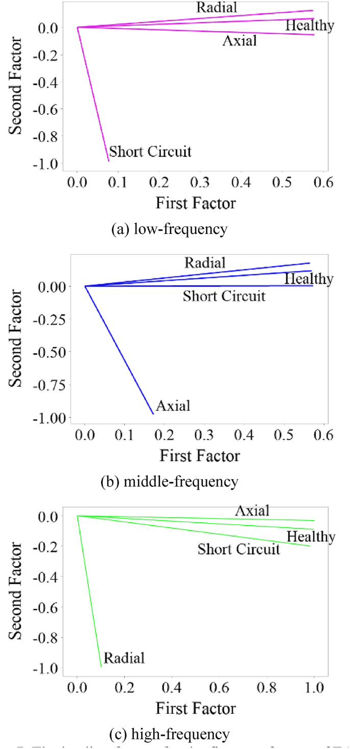
The loading factors for the first two factors of FA. (a) low-frequency, (b) middle-frequency, (c) high-frequency.

In the mid-frequency range (Fig. 7b), the variables divide into healthy systems and SC, AD, RD defects. Here, the SC and RD data match healthy system data, whereas FA fails to establish this correspondence for AD cases. At high frequencies (Fig. 7c), the classification yields healthy systems versus SC, AD, and RD systems. While the SC and AD data correlate with healthy system data, FA does not demonstrate this correlation for RD cases.

C.3. Results of FCA to indicate winding faults

The findings of FCA to detect transformer winding defects are provided in this section. As illustrated in Figs. 8a-c, the variables can be classified into two groups according to their frequency characteristics. At low frequencies (Fig. 8a), the classification reveals: (1) healthy, AD, and RD systems, and (2) SC systems. Accordingly, the AD and RD values closely match those of healthy systems, while FCA does not demonstrate this correspondence for SC cases. In the medium frequency range (Fig. 8b), the groups comprise: (1) healthy, SC, and RD systems, and (2) AD systems. Here, the SC and RD values align with healthy system values, whereas FCA fails to establish this relationship for AD data. At high frequencies (Fig. 8c), the classification yields: (1) healthy, SC, and AD systems, and (2) RD systems. While the SC and AD measurements correspond to healthy system values, FCA does not confirm this similarity for RD data.

Fig. 8

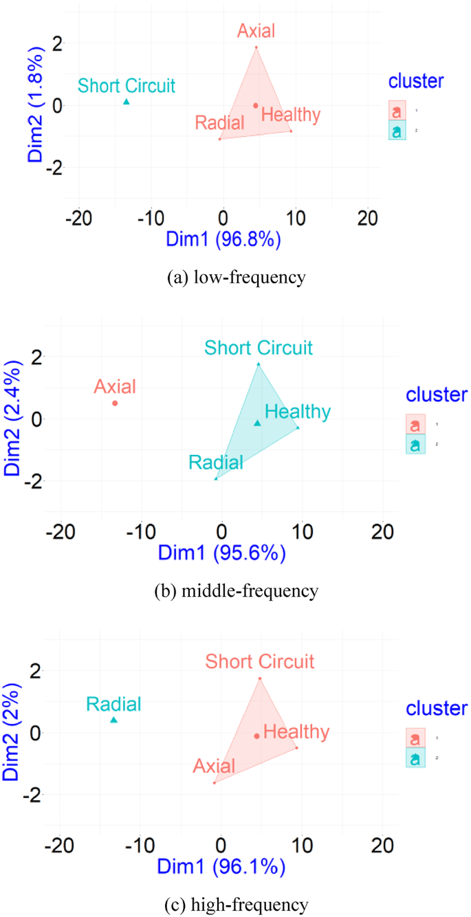
Fuzzy clustering plot. (a) low-frequency, (b) middle-frequency, (c) high-frequency.

Comparative analysis

In this section, we provide a comparative analysis of our proposed methods against several alternative methods, including random forest (RF)41, artificial neural network (ANN)42, gradient boosting (GB)43, and decision tree (DT)44. The evaluation is based on four key performance metrics: precision, recall, F1-score, and accuracy by the following formulas:

and

.

where TP, FP, FN, and TN denote True Positives, False Positives, False Negatives, and True Negatives, respectively. As it can be seen in Table 5, our data visualization approaches outperformed all comparative methods in terms of most performance metrics. The FCA approach achieves the highest accuracy, with 98.9, outperforming all other methods.

FA, PCA and RF acts approximately similar with accuracies 96.6%, 96.6% and 96.4%, respectively. Although the performance of RF is similar to PCA and FA, but since PCA and FA are visual approaches, we recommended these techniques instead of RF. The results from the comparative analysis clearly demonstrate that our proposed visualization approaches outperform alternative methods across all evaluated metrics. This consistent superiority of our methods highlights their potential as more reliable and effective solutions for the problems at hand.