Like many people who are just getting started with Excel, I used to think it was just about rows, columns, and formulas. You know — the basic stuff. For years, I spent countless hours copying and pasting data to unpivot it. This was tedious, error-prone, and frankly exhausting to do, especially when dealing with large datasets. But through research and a bit more experience, I discovered that Get Data has a feature that changed how I deal with pivoted data.
I no longer have to make endless manual adjustments to get data in the format I need. Excel does all the heavy lifting with this simple button. What once took hours now takes minutes. Furthermore, the result is cleaner, more reliable, and easier to analyze. It was a shame I didn’t learn about it sooner.
Manually unpivoting data sucks
Manual data preparation takes a long time
When I started working with data from different sources, such as sales reports, financial statements, and survey results, I felt the pain of dealing with pivoted data. You get pivoted data when you organize categories as column headers, with the corresponding values arranged beneath them. This arrangement creates a wide table format that makes comparisons easier. On the downside, it makes data analysis more difficult.
To fix this, I would create a new sheet and copy and paste values into it. This involved manually rearranging columns to match the required data analysis format. Afterward, it was a matter of repeating the process whenever new data arrived.
![]()
Related
I Used to Hate Cleaning Excel Data—Now I Look Forward to It
Yes, my relationship with dirty data took an unexpected turn.
The biggest problem is that the inefficient manual process increases the risk of errors. In critical Excel sheets, even a tiny mistake can throw off the entire data analysis. This is why finding a better way to unpivot data felt like a revelation.
Instead of bending over backward to clean messy Excel data so it works well with formulas, I realized I could reshape the data itself—automatically, consistently, and without errors.
How the Get Data button gave me what I needed to unpivot data
It was the game-changer I needed
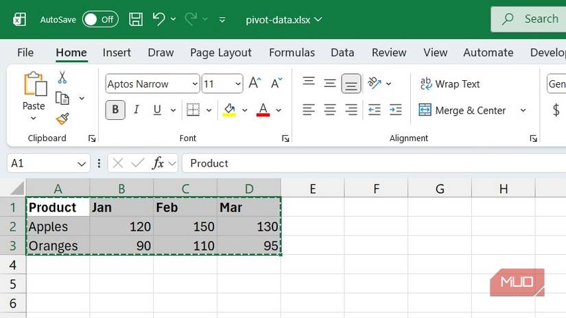
Let me set the scenario to show why unpivoting data is such a big deal. Imagine you have a table with one column per month — January, February, March, and so on. Here’s what the table would look like:
Product
Jan
Feb
Mar
Apr
Apples
120
150
130
140
Oranges
90
110
95
100
While this layout looks fine, it isn’t ideal for data analysis because Excel treats the months as separate columns rather than as values you can filter or group. Suppose I wanted to draw a chart from the data showing sales over time. Excel would struggle to do so because the months are headers rather than data points that should appear on the chart.
For the data analysis to work, the table needs to look something like this:
Product
Month
Sales
Apples
Jan
120
Apples
Feb
150
Apples
Mar
130
Oranges
Jan
90
Oranges
Feb
110
Oranges
Mar
95
The months are now properly listed in a column called Month, and the sales are in their own column, too, called Sales. This is a structure that data analysis tools, such as formulas, charts, and pivot tables, find easier to work with. Achieving this only takes a few clicks, thanks to the Get Data feature.
How I use the Get Data button to unpivot data
No need to write complicated formulas
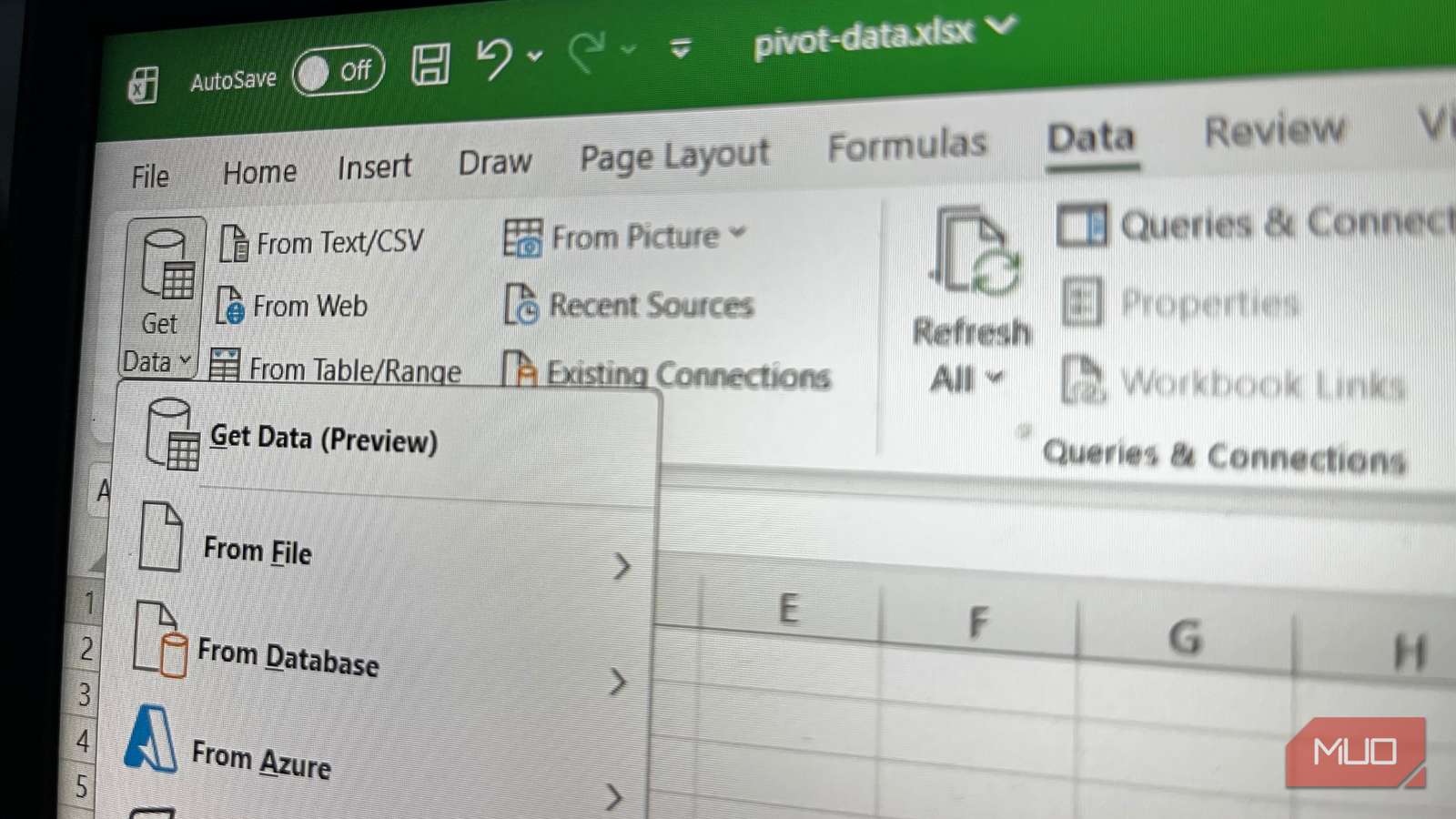
Continuing with the data above, unpivoting is laughably easy using the Get Data button. All I have to do is click Get Data -> From Other Sources -> From Table/Range to open the Power Query editor. This option is ideal when the data has already been loaded. However, there are several other data sources to choose from if needed (e.g., another Excel sheet or an Azure database).

Related
I Finally Tried This Excel Feature Everyone Knows But Ignores—It’s Much More Useful Than I Thought
The underdog Excel feature that deserves your attention.
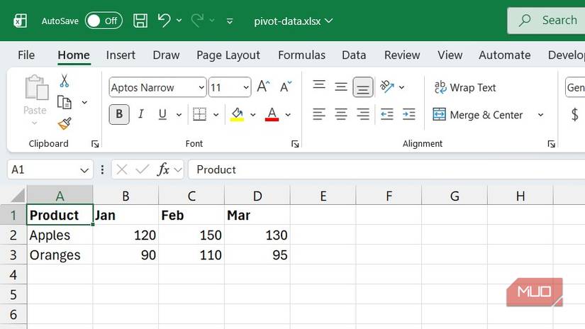
Since the data isn’t in a table, Excel will prompt you to convert it to a table before opening the Power Query editor. Afterward, I can select all the columns I want to unpivot — these are the columns with the months. From there, unpivoting the data is a matter of choosing the Transform tab and clicking Unpivot columns.
Unpivoting will place the month names in one column and the corresponding sales data in another. The new columns can be renamed to Month and Sales from within the Power Query editor. From there, I can do other Power Query operations, such as filtering out unnecessary rows and performing additional data transformations.
Finally, selecting the Home tab and clicking Close & Load creates a separate Excel sheet with the unpivoted data. Everything will now be ready for analysis.
I am never going back to copy-pasting data to unpivot it
The “Unpivot” button inside Excel’s Get Data feature is a hidden superpower. It can turn a tedious, error-prone task into smooth, automated workflows. No more copy-pasting, no more manual rearranging — unpivoting ensures the data is in the right structure for the job. Now, when I see pivoted data, I no longer reach for Ctrl + C and Ctrl + V.