Table 3 provides descriptive statistics of the variables under study. These statistics provide an overview of the mean, median and standard deviation of the sample. Furthermore, it also shows skewness and kurtosis and the Shapiro-Wilk test value for normality. The above table shows the statistics of IDC, CE, AI, economic growth, research and development and trade openness. The mean values of IDC and TOP are higher than median; the standard deviation of IDC is higher than both mean and median (SD = 10.2958), while the standard deviation of TOP is lower than mean and median (SD = 58.998). IDC is right-skewed distribution with high variability while TOP mild right-skewed distribution with very low variability (SK = 2.0022, 1.7351), the high kurtosis values for IDC (6.5624) and TOP (7.3507), signify heavy tails, though normality is rejected (p < 0.05).
Conversely, the mean and median of CE and AI is almost zero and standard deviation is higher than mean and median (SD = 0.9522, 0.9714) which shows symmetric distribution and exhibits both moderate variabilities, though normality is rejected by shapiro-wilk (p < 0.05). GDP and R&D have almost same mean and median and standard deviation (SD = 4.0731) of GDP is higher than mean and median while standard deviation (SD = 0.9040) of R&D is lower than mean and median, though the normality is rejected. The Skewness of CE, AI an R&D is positive while GDP is negative (SK = 1.0467, 0.1776, 0.7269, −0.1309). On the other hand, kurtosis of CE and GDP is greater than 3 which indicates platykurtosis behavior while AI and R&D have less than 3 which indicates leptokurtic behavior. Figure 2 shows IDC across EU Countries. The yellow region shows high industrial de-carbonization countries; the brown color region shows median industrial de-carbonization countries, and the red color region shows low industrial de-carbonization countries.
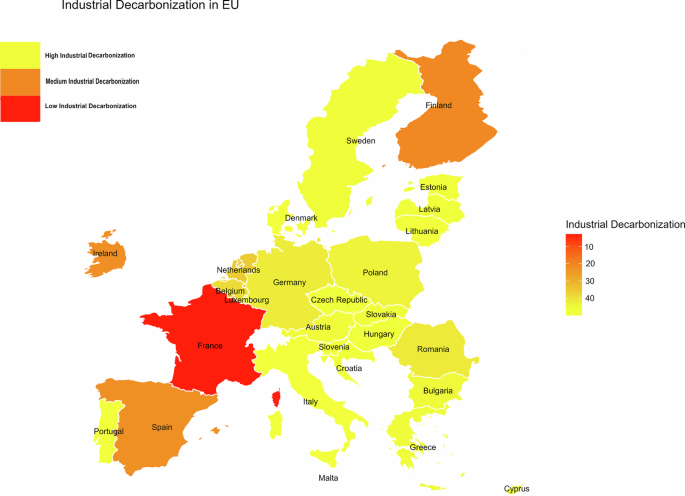
Industrial decarbonization.
Time-specific heterogeneous factor analysis
This study employed TSHFA, an advanced econometric technique to develop two novel indices CE and AI. TSHFA is optimally designed to analyse panel datasets, allowing for the shifting dynamics and multi-directional relationships between variables over time. Time-specific heterogeneous factor analysis is an advanced econometric and statistical methodology used for identifying latent common factors in panel data, while explicitly addressing heterogeneity across cross-sections and time. TSHFA diminishes the assumptions of homogeneity and stationarity used in traditional factor analysis or principal component analysis by allowing factor loadings and relationships to vary over time. This makes it especially useful for developing indices from panel datasets that may experience structural changes, country-specific shocks, or technological changes. The CE index is constructed from 7 variables and AI index from 5 variables that capture fundamental aspects of CE and AI were used. Figures 3 and 4 show KMO (Kaiser-Meyer-Olkin) test results for factor analysis, the results show that KMO values vary between 0.0 and 0.8, values closer to 1 represent strong sampling adequacy which implies all the variables of CE and AI are useful for factor analysis. Figure 5 depicts the year-wise comparison of the CE index for the years 2000 to 2023. The changes in the graph demonstrate a change in value of CE over a period of time, which indicates positive or negative change in resource use efficiency, waste management, and sustainability. The graph also shows the progressive changes in the CE index efforts throughout the years in the given period. As shown in Fig. 6, the year-by-year pattern of the AI is reflected in the 2000 to 2023 timeframe. Changes in the graph reflect the trend of innovation forecasts, technology adoption, and R&D investment in computer technology, establishing whether AI is on a positive, neutral or negative trajectory in a period of time. This clarifies the processes associated with AI with respect to the precision of timeframes and its future impacts.
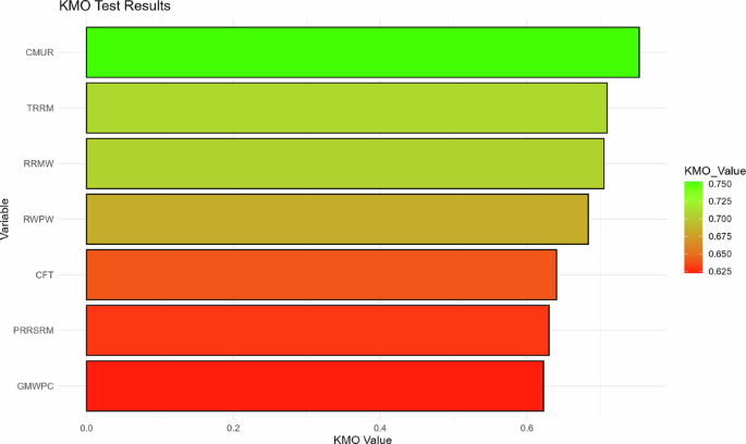
KMO test result of circular economy.
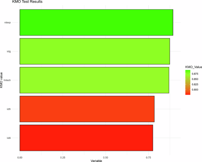
KMO test result of artificial intelligence.
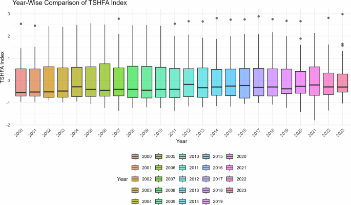
Year-wise comparison of circular economy index-I.
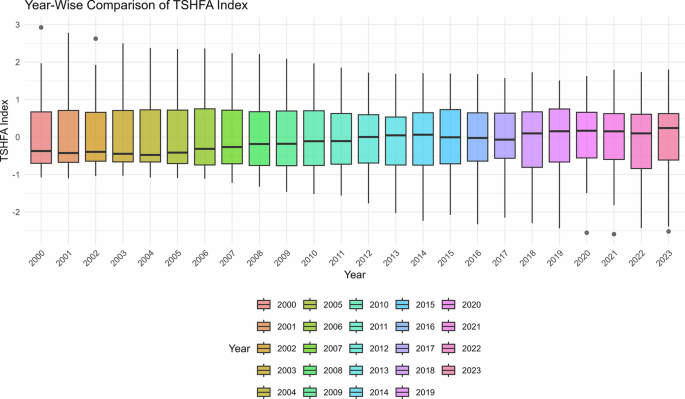
Year-wise comparison of artificial intelligence index-II.
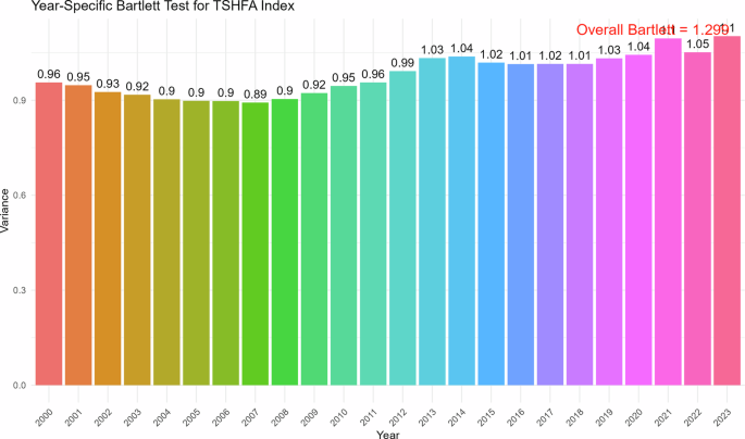
Figures 7 and 8 provide results of the Bartlett test for different time intervals, which provide evidence of the sphericity of the data that were utilized for constructing the CE and AI index. The values shown above the bars in Figs. 7 and 8 correspond to the graphical illustration of the Bartlett test for all time intervals, which proves the construction of the indices to facilitate robust verification of the processes. Figures 9 and 10 provide the scree plot for the overall index, which reveals the ideal number of indices which could be generated from the variable set. The line is on a significant decrease from 2 to 3, which suggests that it is best to construct index from different variables. Figures 11 and 12 present the temporal changes in the CE and AI factor loadings of different indicators. This makes it easier to understand how the CE and AI factor loading scores changed over time. This is the new feature of this heteroskedastic factor analysis method and evolving patterns reveal how the significance of each variable shifts over time, are features of method called time heterogeneous factor analysis. The chart captures changes in the CE performance alongside AI adoption, providing deeper multidimensional insights into the interconnected trends.
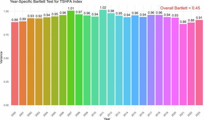
The Index-I of circular economy year-specific Bartlett test result.
Index-II of artificial intelligence year-specific Bartlett test result.
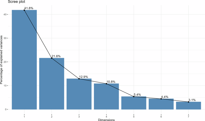
Scree plot of Circular Economy Index-I.
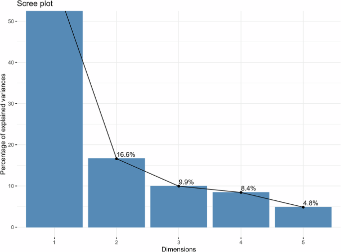
Scree plot of Artificial Intelligence Index-II.
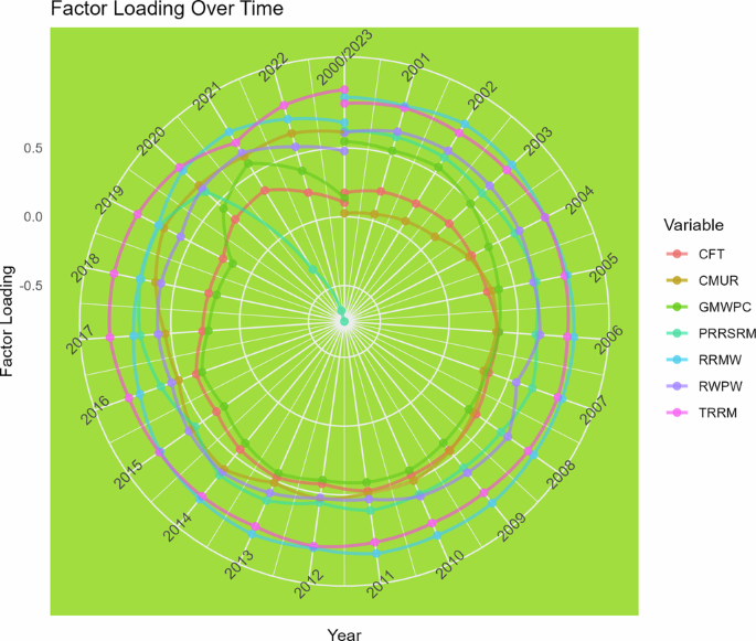
Factor loadings of the CE-Index overtime.
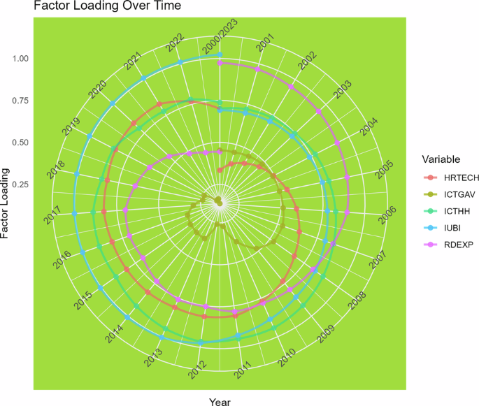
Factor loadings of the AI-Index overtime.
Panel unit test: CIPS and CADF
Upon confirming the presence of CSD in the dataset, the subsequent step is to assess the stationarity of the data. The CSD results validate the presence of cross-sectional dependence in the dataset. The second-generation unit root tests (CIPS and CADF) were employed due to the inadequacy of first-generation unit root tests in addressing cross-sectional dependency and heterogeneity. Table 4 display the results of the second-generation unit root test (CIPS and CADF). The cross-sectional IPS result reveals that nearly all variables are stationarity at the first difference level except GDP which is stationary at the level, indicating a mixed order of integration. CADF validates that all variables are stationary at the first difference level. The results of CIPS and CADF should assurance the credibility and dependability of subsequent econometric procedures like co-integrative or causative examinations.
Co-integration test
Table 5 display the results of panel co-integration tests from Westerlund and Edgerton (2008) and Pedroni (2004) to validate the long-term equilibrium relationship among the variables. The Pedroni test results reveal that: The Modified Phillips–Perron t-statistic is highly significant (6.0354, p = 0.000), strongly suggesting the rejection of the null hypothesis of no co-integration, the Phillips-Perron t-statistic (−12.371, p = 0.000) and ADF t-statistic (−10.514, p = 0.000) are also significant at conventional levels, indicating stronger evidence for co-integration when considered independently. The substantial Westerlund test statistic (p < 0.05) provides evidence of co-integration, enabling the interpretation of long-run coefficients from the PQR-PMG and PQR-CCE models. The results indicate the presence of co-integration among the variables.
Correlation matrix
Table 6 illustrates the correlation matrix among industrial de-carbonization, CE, AI, economic growth, R&D and trade openness. All variables exhibit a positive link with industrial de-carbonization, with the exception of economic growth and trade openness, which demonstrates a negative correlation. The lack of significant correlations, all under 0.5, indicates the absence of serious multi-collinearity problems, hence validating the inclusion of these variables in the study. Table 6 also display the result of variance inflation factor (VIF) which shows that VIF value is less than 5 (mean VIF = 1.24) it means there is no multi-collinearity exists among the study variables.
Cross-sectional dependence test
Table 7 presents two varieties of cross-sectional dependence (CSD) tests to evaluate CSD within the panel data set of EU countries. The two categories of CSD tests are Pesaran (2004) and Friedman (1937); the outcomes of these tests provide compelling evidence for the existence of CSD. The Pesaran (2004) test yielded a statistically significant result (9.761, p = 0.000) at the 1% level, so affirming the rejection of the null hypothesis and providing robust evidence for the presence of CSD. The Friedman (1937) test statistic yielded also to reject the null hypothesis of independence (86.007, p = 0.000), indicating strong evidence cross-section dependence. The results are indicative, relying on the substantial findings of Pesaran and Friedman, which demonstrate that the dataset exhibits cross-sectional dependence. Table 7 additionally display the results of the slope of heterogeneity, confirming that the values of ΔSH and adjΔSH provide substantial evidence of heterogeneity within the panel data set. The p-value is markedly significant and substantiates the rejection of the null hypothesis.
Panel quantile regression-PMG results
Table 8 exhibits the PQR-PMG long-run estimates at different quantiles. The results shows the long-run effect of CE, AI and the moderation effect of AI between CE and IDC across different quantiles in EU region. The results indicates that when there is a 1% increase in the CE in the EU region, the estimates associated with CE went from 0.93 at the 25th quantile to 9.1 at the 90th, suggesting that CE practices contribute a greater impact to IDC in EU countries with higher level of IDC and as we move toward the upper quantiles the size of the effect gets bigger. The positive effects of CE, AI, and particularly the interaction (CE*AI) are quite strong at the higher quantiles (75th and 90th), highlighting that in more advanced or more carbon-intensive regions, CE and AI provide greater support to improve IDC. This trend indicates that countries which are already in decreasing carbon emission experience higher marginal benefits from these technologies and strategies. One possible reason: these countries have the advanced sustainable infrastructure, technological maturity, a skilled workforce, and a regulatory environment to effectively absorb and implement CE practices and AI technologies. Thus, the efficiency improvements and emission reductions that these technologies may realize would be further pronounced in these contexts. The results align with the results of (Hailemariam and Erdiaw‐Kwasie, 2022) present strong empirical evidence that CE growth plays a significant role in improving environmental quality through the reduction of CO₂ emissions. Similarly, Bressanelli (2025) also support our finding that how manufacturing companies adopt CE practices to decrease carbon emission and is widely varied and depends on the systematic change across a number of industrial areas. He employed a pragmatic tool for measuring industrial circular practices first, and then links to actual reductions in carbon footprints, knowing that CE implementation generates variable benefits attributed to varying levels of CE practices.
AI exhibits strong positive effect on IDC at all quantiles and is even larger at higher quantile levels, underscoring the pivotal role of AI in enhancing IDC and increase the environmental quality. The result of AI on IDC aligns with the result of (Zhong et al., 2024), AI can reduce carbon emission and confirms the importance of industrial and demographic structures in promoting carbon emission reduction. The interaction of AI with CE practices (CE*AI) has strong positive impacts at all quantiles and grows towards the upper quantiles (values vary from 0.49 to 3.59). This suggests that AI alone significantly enhance IDC while also moderate the relationship between the CE practices and IDC in EU region. The results of the joint effect of CE*AI align with the findings of (Zhang et al., 2025), quantifiable emission reduction effects arising from the integration of these approaches particularly in leading decarbonizing economies. These findings are in line with earlier studies which pointed to the relevance of the implementation of the CE paradigm and Artificial intelligence towards sustainable development.
Conversely, TOP (Trade Openness) has a persistent negative effect at all quantiles. This suggests that 1% increase in TOP causes the decrease in IDC, this is likely a function of structural trade. The negative impact of limited value-added type exports and structural trade difficulties is indicated and supported by recent evidence of trade vulnerabilities in recent scenarios open economies. This dynamic is particularly relevant in the EU’s complex industrial supply chains, where openness can simultaneously drive economic benefits and environmental challenges. The result is similar with the finding of (Derindag et al., 2023). Conversely, R&D exerts a substantial and positive influence, at lower signifying that technology investment is essential for facilitating advancements in de-carbonization. However, at median becomes negative and at higher quantiles 75th, indicating diminishing returns, possible inefficiencies and rebound effects when technological advancements result in increased emission. This result is similar to that of (Mamkhezri and Khezri, 2024). GDP is insignificant at all quantiles. This could be an indication of saturation effect, where ongoing economic growth in high-income countries is not producing proportional improvements to the environment. This insignificant results of economic growth are similar to those of (Abd El-Aal, 2024), which empirically shows that economic growth exhibits insignificant with carbon emission in high-income countries.
Having examined the effects of these variables, the question arises: how can these factors be effectively leveraged to enhance IDC? To address this, the study provides dynamic factor loadings in Figs. 10 and 11. The magnitude of these factor loadings reflects the relative contribution of each variable to the overall outcome. Notably, CE and AI emerge as critical drivers, particularly at higher quantiles, emphasizing their potential to drive transformative change. The coefficient in the overall model is both significant and positively correlated, pointing to a baseline improvement in the IDC. This implies that the model captures an inherent underlying effect, reinforcing the reliability and strength of the findings.
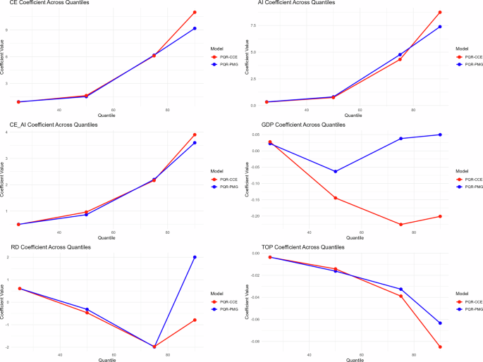
Panel quantile regression-CCE results
Table 9 shows the CCE heterogeneous effect at different quantile. The CCE results reveal heterogeneous effects of the CE, artificial intelligence (AI) and interaction term (CE*AI) across the 25th, 50th, 75th, and 90th quantiles. The effect of CE, AI and their interaction (CE*AI) are not the same at different points of the conditional distribution of the IDC in EU region. At lower quantile 25th CE and AI have positive and significant effects, although the sizes are small which implies that countries that are relatively early in the process of de-carbonization can receive some positive benefits, but the benefits are not large. At median quantile 50th CE is slightly high and AI is insignificant and mostly the interaction CE*AI drive the IDC. This suggests that using CE and AI in combination, in the median quantile the use of these strategies is more powerful than using either CE or AI alone. The positive effects of CE, AI, and particularly the interaction (CE*AI) are quite strong at the higher quantiles (75th and 90th), highlighting that the more advanced or more carbon-intensive regions, CE and AI provide greater support for IDC. In essence, the heterogeneous effect underscores that CE and AI are not uniformly influential; instead, their effectiveness strengthens in high-emission, while their standalone effects are weaker at the lower and middle quantiles. The results of heterogeneous effect of CE aligned with the finding of (Wang et al., 2023) who studied the heterogeneous of CE on carbon emission in top 7 carbon emission countries, they indicate that CE have positive association with carbon emission in designated countries. These results of heterogeneous effect of AI are similar to the findings of (Zhong J et al., 2024), investigated the heterogeneous effect of AI on carbon emission in 66 global economies, they present that AI effect varies across different regions its effect increases in places with older population. Trade openness (TOP) shows the negative significant effect at all quantiles. This negative effect is stronger at upper quantiles which means that greater TOP associated with higher carbon intensity specially in countries with higher carbon emission. Conversely, R&D exerts a substantial and positive influence, at lower signifying that technology investment is essential for facilitating advancements in de-carbonization. However, at median becomes negative and at higher quantiles 75th, indicating diminishing returns, possible inefficiencies and rebound effects when technological advancements result in increased emission. GDP is insignificant at all quantiles. This could be an indication of saturation effect, where ongoing economic growth in high-income countries is not producing proportional improvements to the environment. These findings highlight that CE and AI adoption are the primary drivers of IDC, trade openness continually hinders de-carbonization, whereas R&D funding is most efficacious at initial stages but diminishes in efficacy as economies progress up the distribution. These results confirm the steady and remarkable impacts of CE, AI, and CE*AI at higher quantiles most especially in having positive. Figure 13 shows that CE, Artificial Intelligence (AI), and their interaction (CE*AI) are increasingly strong positive effects in regard to higher quantiles, emphasizing that they are more responsible for improvement in a region with higher levels de-carbonization., Gross Domestic Product (GDP) showed mixed effects, it was positive in PQR-PMG but predominantly negative in PQR-CCE but insignificant. Research and Development (R&D) has mixed effect, being positive at the lower quantiles, then turning negative in between quantiles, then being of benefit at the top quantile’s lows, this suggests that R&D may have differing effectiveness depending on the level of development of a society. Trade Openness (TOP) showed negative effects consistently, even worsening at higher quantiles, this suggests a potential environmental cost of being open to trade. Both CE, AI and the interaction of both, you can conclude that CE, AI, and CE*AI are responsible for sustainable improvement, while GDP, R&D, and TOP have relatively more complicated or adverse effects in respective contexts.