Operationalizing the environmental safe operating space into target distributions for mobility and batteries

Based on recommendations and learnings from literature50,51 and to align with the functional unit definition in LCA52, we select “per pkm” as the target metric for passenger mobility. We define our system boundaries as encompassing both cradle-to-grave (for the vehicle) and well-to-wheel (for the fuel or charging of batteries). For batteries, we select “per kWh battery capacity” as our target metric, since it eases comparability between different chemistries, sizes and energy densities50,53,54. Therefore, system boundaries for the battery targets only comprise manufacturing (cradle-to-gate), which could include recycled content.

Defining safe operating spaces

Within the PB framework, the nine boundaries are quantified via control variables, which represent the most significant drivers leading to the perturbation of a specific boundary18. Then, SOS are defined from the control variables values which safeguard the resilience of the Earth system18.

Dependent on methodologies for control variable approximation and the targeted state of the Earth system, various possible SOS for anthropogenic activities can co-exist14. Here, we select the PB-LCIA methodology which proposes to link the PB-SOS to LCIA by multiplying elementary flows by their normalized individual contribution to the safe operating budget55. We also compare PB-SOS against the SOS obtained from the carrying capacity approach, via sustainable living normalization factors for an egalitarian distribution of global impacts per capita56. Specifically for climate change, we consider RCBs as other potential SOS, since they prescribe the amount of CO2-eq that can be emitted to limit the elevation of the planet’s temperature to a fixed threshold (e.g., 1,1.5 or 2 °C).

Safe operating space for climate change

Two control variables can express the PB for climate change: (1) an atmospheric CO2-eq concentration of 350 ppm and/or (2) a radiative forcing of 1 W/m2. Both control variables aim to limit further warming and to restore Earth’s energy balance at a temperature increase of around +1 °C in comparison to pre-industrial times57,58. Due to current concentration overshoot (the atmospheric CO₂ concentration averaged 424.61 ppm in 2024 at the Mauna Loa Observatory59), we cannot treat the 350 ppm CO₂ control variable as a remaining budget that can simply be divided over future years, since this would lead to negative budgets. Following Steffen et al.2’s SOS definition and Ryberg et al. 55’s PB-LCIA approach, we use the full SOS for anthropogenic activities defined as the difference between 350 and 278 ppm (i.e., 72 ppm), the latter being the natural background level of CO2 in the atmosphere60.

Based on the mid-term (2000–2300) representative concentration pathway (RCP) 2.6, Ryberg et al. determined that each kilogram of CO2 emitted annually corresponds to a steady-state increase of 2.69 × 10−11 ppm in global atmospheric carbon dioxide concentration55. For example, a climate-change result of 0.1 ppm CO₂ for a given functional unit means that the continuous annual GHG emissions associated with performing that activity would in a certain way, over time, lead to a steady-state increase of 0.1 ppm in atmospheric CO₂. Relative to the full SOS of 72 ppm, this corresponds to occupying about 0.14% of the available space. Abiding to that definition, we do not assume that the 72 ppm SOS is an unused stock that can be allocated directly as an annual allowance; rather, it is used as a reference to express the share of the full SOS occupied by the product system. Whether this share is acceptable or not then depends on how the SOS is downscaled to the level of the activity. Since the current state of the Earth System is above 350 ppm, to return within the planetary boundary, all human activities have to fit within 72 ppm, where cumulative pressures would start to decline back toward the boundary on the long-term. Converting 72 ppm to kg CO2-eq/yr (with a conversion factor of 2.69 × 10−11 ppm∙yr/kg CO2-eq55) yields a global budget (SOSglobal) of 2.68 × 1012 kg CO2-eq/yr. Then, selecting an egalitarian approach, which is coherent with all other explored SOS, we divide the budget by the projected global population in 2030, 2035 and 2050 to provide individual SOS for climate change, listed in Table 3. We use world population prospects provided by the United Nations’ medium fertility variant for 2024 onwards36.

As comparative safe operating spaces, the carrying capacity-LCIA method of Bjørn et al. proposes normalization factors of 522 kg CO2-eq/capita to limit radiative forcing at 1 W/m2 or 985 kg CO2-eq/capita to limit temperature increase to 2 °C56. Since these equal per capita factors were calculated with the global population in 2010 (valued at 6.9 billion56) we update them by replacing the time dependent population denominator with prospects for 2030, 2035 and 2050 (reported Table 3).

Lastly, we explore RCBs as SOS for anthropogenic activities. In comparison to both PB and carrying capacity approaches which are static, that is, defining a fixed annual emission threshold to reach a targeted long-term equilibrium state, RCBs are dynamic in nature10. A dynamic approach defines an evolving annual boundary (GtCO2-eq emission limit) based on a cumulative calculation and a linear reduction in order to stay on the trajectory to meet net-zero10. We propose a deep dive into the RCB of 1150 GtCO2-eq starting in 2020, for a 50% probability of limiting the Earth’s temperature increase to 2 °C by 210011. We selected a scenario which limit temperature increase to 2 °C, since in 2020, it is highly likely that the Earth entered the 20-year period experiencing a temperature increase over 1.5 °C61,62. Corresponding calculations to convert the RCB into annual safe operating spaces for 2030, 2035 and 2050 are based on the methodology proposed by Clausen et al.10, assuming linear reduction in annual emissions until net-zero occurs. Therefore, the year to net-zero determines the annual allowable carbon budget. The resulting individual SOS budgets presented in Table 3 consider a first net-zero year in 2070. We also consider an alternative pathway, wherein year 2060 is rather set to measure its influence on targets at the battery pack level (found in Supplementary Data T3).

Noticeably, the RCB-based individual carbon budget in 2030 (for a 50% probability of limiting temperature increase to 2 °C) is much more permissive than the SOS determined by the PB-LCIA ( + 1550%) or by the corresponding carrying-capacity based approach ( + 600%), with a similar trend observed in 2035. In 2050, the reported differences decrease to +800% and +250%. Time independent (i.e., static) safe operating spaces are listed in Table 4 to ease updatability for future scenarios (i.e., dividing by new population prospects). The difference in quantified safe operating spaces via the PB-LCIA and carrying-capacity-LCIA approaches for a radiative forcing of 1 W/m2 (or limiting to 1 °C increase) is explained in the varying procedures to calculate the long-term radiative forcing of CO255,56.

Safe operating space for freshwater use

During the third assessment of planetary boundaries in 202318, the water PB was updated from the previous 4000 km3/yr of blue water use to a new version proposed in terms of streamflow and soil moisture63. The updated definition suggests a limit on global land area – 10.2% for streamflow (blue water) and 11.1% for soil moisture (green water) – which experience local deviations occurring naturally once in 20 years in the pre-industrial reference state63. As a reference point, these limits are currently being transgressed for 18.2% and 15.8%18 of global land area for blue and green water respectively. As a safe boundary for surface water deviation, Rockström et al. propose to limit monthly flow alterations to 20%64. Aggregating this condition at the global level yielded a maximal altered flow of 7600 km3/yr, much higher than the initial boundary of 4000 km3/yr, due to the revision of world annual runoff considering newly accessible water from the Amazon, the Congo and the high arctic regions with a warming climate64. Aggregating the 20% condition with previous estimates for world runoff yielded an SOS of 2500–3260 km3/yr64.

Until consensus is reached on how to translate maximal flow deviations into freshwater use, we select 2800 km3/yr65 as an extremum that should only give an indication of the maximal water intake66. To note that 2800 km3/yr represents the maximal volume of water that can be withdrawn from freshwater bodies, regardless of being returned or not to its outtake. Consumptive water use, which considers only the fraction of water that is not returned to the environment, is estimated at ~1800–2100 km3/yr for all human activities66. To convert the global freshwater use into a per capita limit, we divide 2800 km3/yr by the projected global population prospects. Resulting individual safe operating freshwater use budgets are reported in Table 5. To create an interval for our sensitivity analysis, we also compute stricter individual freshwater use limits from the carrying capacity budget of 2100 km3/yr56.

Our approach is non-scarcity-weighted, i.e., it assumes that 1 m³ of freshwater withdrawal has the same impact regardless of location. We did not adopt a more spatiotemporally resolved method such as watershed-level safe operating spaces67 mainly because the upstream supply chain of electric car batteries is global, and supplying regions will vary over the years. However, if all supplying regions are known, spatiotemporally resolved operating spaces can generate a more actionable target. Based on regional water scarcity indicators, deprivation-weighted water consumption can be considered instead of simple water withdrawal42,68. Following that approach, a global deprivation limit of 182,000 km3 worldeq/yr can be distributed equally per capita42. We performed such alternative and provide scarcity-weighted targets in Supplementary Data T10.

Procedure for downscaling

Five levels of allocation are considered in our proposed methodology (refer to Fig. 6) where we also provide an overview of the target metrics at various downscaling levels in Table 6:

1.

National scaling, from the global SOS to a specific country, where possible enacting metrics are population, inverse GDP, cumulative historical emissions and current national emissions to downscale the SOS to a specific country based on egalitarian, ability to pay, historical contribution and acquired rights approaches respectively. In this study, we only considered an equal per capita approach.

2.

Sector scaling, from national SOS to mobility sector, where emission grandfathering and sufficiency-based allocation factors are used to downscale the national budget to the mobility sector.

3.

Sub-sector scaling, from mobility to passenger cars contribution, where both grandfathering and sufficiency-based sharing principles are compared to determine the split between different mobility options (such as air, rail, buses and cars).

4.

Product scaling, from the passenger car fleet to one electric vehicle, where the number of vehicles in the national fleet is considered based on an acquired rights principle to facilitate the allocation.

5.

Component scaling, from an electric vehicle to its battery, where we use prospective LCA scenarios based on emission grandfathering to provide a maximal share for batteries. Note that for water use, level 2 had to be skipped, as no information is currently available for the share of mobility. Therefore, the allocation procedure jumps from level 1 to level 3, as detailed in the corresponding section on specificities of sub-sector allocation for freshwater use.

Fig. 6: Overview of the proposed methodology to downscale sustainability targets for life cycle passenger mobility.

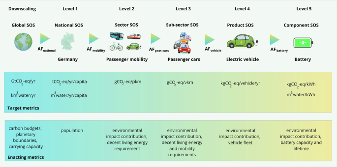
Illustrated with climate impacts and water use, global safe operating spaces (SOS) have units in Gt CO2-eq/yr and km3 water/yr, which are defined by the enacting metrics of carbon budgets, planetary boundaries or carrying capacity limits. Downscaling first to a national level, target metrics are divided by capita following an egalitarian approach, using the share of global population as enacting metric. For Germany, the corresponding allocation factor is 1% of the global population. Level 2 of downscaling is at the sectoral level, in this case mobility. Sectoral allocation is defined via decent energy needs or historical environmental impacts. Level 3 corresponds to a sub-sector, in this case passenger cars, where again both decent energy needs and historical environmental impacts can be used to compute an allocation factor. Level 4 of downscaling corresponds to a product, in the present study an electric vehicle, where the allocation is performed by considering a number of cars in a national fleet. For water use, historical data on water consumption of the existing car fleet is also required for the allocation to one car. Finally, we stop our downscaling at level 5, corresponding to a product component, in the present case the battery pack of an electric car. For such allocation, estimations of the battery’s environmental impact share, its capacity and lifetime are required to allocate a target per kWh.

Downscaling to a national level

In the present work, global safe operating spaces (i.e., SOSglobal) are simply multiplied by the proportion of the current or projected population of a country against the worldwide population (AFnational), coherent with an egalitarian approach (refer to Eq. 1). Germany and Canada are selected as a first case study, in order to assess resulting climate impact and water use targets for countries that currently heavily rely on passenger cars for mobility23,24. We use population prospects (POPnational) for Germany, Canada and the world provided by the United Nations’ medium fertility variant for the years 2030, 2035 and 205036.

Downscaling to the mobility societal sector (target in g CO2-eq/pkm)

Downscaling at a sectoral level is only performed for climate change in this study. Water use targets are non-calculable for the mobility sector due to enacting metric data being unavailable. Therefore, mobility solutions cannot be benchmarked against an SOS-based water use target per pkm where water usage can only be compared in conventional LCAs.

In 2023, the transport sector (excluding other transport and international shipping) contributed to 26.1% and 22.1% of national GHG emissions for Germany and Canada respectively (reported according to Article 13, paragraph 7(a), of the Paris Agreement69, refer to Supplementary Data F1a). However, since the contribution also includes the transportation of goods, it was not possible to segregate the share of mobility from the reported data. It is estimated that 55.5% of transport emissions are caused by passenger mobility (refer to Supplementary Data F1a). Alternate sources, such as Climate Trace70, report the share of transport sector (excluding other transportation, domestic shipping, and international shipping) for Germany and Canada in 2024 at 15.5% and 17.3% respectively (refer to Supplementary Data F1a). Due to these reported differences and inability to assign a share of transport emissions to mobility, we decided to perform the allocation based on decent living energy needs for mobility as estimated by Millward-Hopkins et al.7. In this approach, location specific information for the mobility sector is provided, where the values for Germany and Canada are at 16% and 26% respectively7. The global average is at 21% (refer to Supplementary Data F1a))7. As a contrast, a more stringent scenario also based on a sufficiency principle estimates at 6% the share for mobility in Denmark68.

To derive a sustainability target at the mobility sector level (g CO2-eq/pkm), the share of SOS allocated to the sector is divided by the average passenger-kilometers traveled per capita each year (\({{\rm{PKT}}}_{{\rm{a}}}\)) for the respective countries (as indicated in Eq. 2).

To assess the impact of the SOSbudget on the resulting mobility target, we conduct a first experiment (reported in Fig. 1a)) where we fix the AFmobility value at 21% (global average) and vary the SOSbudget values from 278 to 5719 kg CO2-eq/capita. We also vary the PKTa value between 5000 and 25,000 pkm/yr based on provided estimates for mobility demand globally7.

Statistical PKTa values for mobility in Canada and Germany are then considered as part of the case study (reported in Fig. 1b)). Pre-COVID 2019 data was selected to reflect the nominal air passenger travel, where the share of PKTa for air mobility in Germany and Canada was 19% and 21% respectively (refer to Supplementary Data F1b). Total PKTa data for Germany24,71 and Canada72 in 2019 were 16,078 pkm/capita and 23,018 pkm/capita (refer to Supplementary Data F1b).

Downscaling to the passenger car sub-sector (target in g CO2-eq/vkm)

To further downscale the target to a sub-sector of passenger car mobility, we require allocation factors for each mode of transport fulfilling mobility requirements. Millward-Hopkins et al. propose allocation factors for five different modes of transport fulfilling all mobility requirements: non-motorized (cycling or walking), road transportation via passenger cars and buses, rail transport and air travel7. Energy demand is distinguished for each transport mode based on direct energy intensity during use stage, and embodied energy in both vehicles and infrastructure. Passenger cars were attributed a sufficientarianism-based share between 14 and 30% of the mobility sector from low and high estimates of energy requirements7 (refer to Supplementary Data F2). In contrast, passenger vehicles (including light-duty trucks) were reported to contribute to 60.7%73 and 53%74 of the German and Canadian transport GHG inventories. Therefore, AFpass-cars were first varied between 20 and 60% encompassing both sufficientarianism and grandfathering approaches (refer to Fig. 2). Then, in our sensitivity analysis on climate impact targets (refer to Fig. 4), both the sufficientarianism (low AFpass-cars = 14%) and the grandfathering principles (high AFpass-cars = 60.7% and 53% for DE and CA) are applied to represent the countries’ current mobility practices.

To derive a sustainability target in terms of VKTa, the share of SOS allocated to passenger cars is divided by the annual travel demand via vehicles for each respective country (as indicated in Eq. 3). The VKTa values of 12,320 and 12,493 vkm/yr were considered for Germany and Canada respectively (refer to Supplementary Data F2). Keeping the target metric on a vkm basis facilitates comparison across drivetrains, wherein the total life cycle emissions of any passenger car can be divided by its total distance traveled and annualized using its lifetime.

Downscaling to a vehicle (target in kg CO2-eq or m3/vehicle/yr)

We estimate permissible life cycle emissions for each vehicle by dividing the national passenger car budget by the total number of vehicles within the country (Nvehicles) (refer to Eq. 4). Since various car sizes and engine types are available in the market, Eq. 4 can be expanded with a weighting factor (Wclass) to arrive at vehicle level targets specific to a particular class of vehicles. The resulting expansion is presented as Eq. 5. Wherein Wclass can be derived either based on ratio of the sum of vehicles in a class (Nclass) multiplied by their respective emission intensity in g CO2-eq/vkm (EIclass) or average weight (AWclass) over the total for all vehicle classes (refer to Eq. 6). Projections of future car fleets are based on a constant occupancy rate of 0.59 and 0.58 vehicle/person in Germany75 and Canada76 respectively, and updated with population projections from the United Nations’ medium fertility variant36 (refer to Supplementary Data T4).

Similarly, vehicle-level targets can be derived for water use by dividing the allocated yearly budget for the passenger car fleet by the number of vehicles. Such targets (in m3/vehicle/yr) based on Eq. 4 and the range of SOS defined in Table 5 are provided for Germany in Supplementary Data T5–DE.

Downscaling to the battery pack (target in kg CO2-eq or m3 water/kWhpack)

For both climate and water use impacts, allocation factors for batteries (AFbattery) were retrieved for two vehicle classes from the carculator20: mini and mid-size vehicles. The carculator estimates prospective impacts of vehicles by modifying life cycle inventories in accordance with predictions from integrated assessment models (IAM), which is streamlined by premise. Therefore, allocation factors for batteries can be retrieved directly from prospective contribution analyses of vehicles for the years 2030, 2025 and 2050. We consider a high and low battery impact factor, where NMC-622 production in China and LFP production in Norway are considered as high and low values. Following the carculator’s projections, the battery capacity increases in time to reflect longer range and improved specific energy of battery packs20.

Building on a previous methodology developed by Ali et al.17, a first Monte Carlo simulation was run to evaluate the sensitivity of climate impact targets (per kWh battery pack) to eleven varying parameter conditions listed in Table 7.

The vehicle lifetime (LT) was calculated by employing a Weibull distribution. The probability distribution was parameterized based on values relevant for Germany, with a shape parameter (β) of 2.4 and a scale parameter (γ) of 14.8 years77. The same parameters are assumed for Canada. The mean vehicle lifetime (μ) was estimated analytically using the gamma function as indicated in Eq. 7, yielding a mean of approximately 13.3 years. Additionally, the 5th and 95th percentiles of the lifetime distribution were computed to define a 90% confidence interval for vehicle lifetimes. The probability density function (PDF) and the survival curve are shown in Fig. 7.

Fig. 7: Determination of the mean vehicle lifetime via a Weibull distribution.

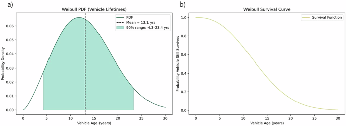
a The probability distribution with a mean of 13.1 years and a 90% confidence interval of 4.3–23.4 years. b The survival curve ending at 30 years.

A total of 10,000 iterations were considered and, in each iteration, the SOSbudget, the allocation factors and the lifetime were independently sampled from uniform distributions defined by their respective literature-informed lower and upper bounds. The product target value, \({{\rm{Target}}}_{{\rm{battery}},{\rm{i}}}\,\)— where i indicates the environmental impact category such as kgCO₂-eq or m3 water used per kWh of battery capacity C — was then computed using Eq. 8.

Uniform independent priors (non-informative in nature) were chosen as a conservative, screening-level assumption that does not prefer any particular value within the reported range. To test the robustness of the resulting target distributions to the choice of prior shape, we performed an additional Monte Carlo analysis in which the parameters (except lifetime) are sampled from triangular distributions with similar upper and lower bounds but with the mode equal to the midpoint of each interval. These results are now provided in Supplementary Data T8.

Furthermore, we also consider a sensitivity analysis on the year to net-zero, by considering it to be 2060 instead of our default assumption of 2070. Details on resulting RCBs are provided in Supplementary Data T3.

To note that for water use targets, the allocation is performed directly from the national budget to the passenger car sub-sector (equivalent to setting AFmobility to 1 in Eq. 3), as detailed in the following section. Monte Carlo simulation parameter values for battery-level water use targets are listed in Table 8.

Specificities of sub-sector allocation for freshwater use

The share of carbon emissions attributed to passenger mobility is widely reported, whereas similar metrics for water use are scarce. Therefore, we calculated an allocation factor for the passenger car fleet directly (without downscaling through mobility), by computing its blue water consumption proportional to the whole water consumption of the country. Most recent total blue water consumption data in the input-output database EXIOBASE 3 for Germany and Canada date from 2022, which we denote as wtotal. Next, the total car stock (i.e., the country’s passenger fleet) (Ntotal) is disaggregated by engine type, where the share of vehicles with engine type j is defined as sj such that \({\sum }_{j=1}^{n}{s}_{j}\,=1.\) In this study, we consider petrol, diesel, EV, hybrid, and hybrid plug-in as engine types, for n = 5. The rest of the engine types are considered to have similar consumption as petrol vehicles. For an engine type j, the water consumption per vkm (wj) is estimated based on the carculator tool20 for the specific countries in the year 2022 to match the EXIOBASE 3’s temporality. With an assumed average annual distance traveled per vehicle (i.e., VKTa), the total water consumption attributable to passenger cars, wfleet, is calculated via Eq. 9.

The allocation factor (AFpass-cars) is then obtained by dividing the water consumption of passenger cars by the total water consumption reported in the EXIOBASE 3 for the year 2022 (wtotal) (refer to Eq. 10).

Equations 9 and 10 provide a simplified approach to estimate the share of water consumption attributed to passenger cars relative to the overall water consumption for the selected regions. Like climate change, we provide low and high AFpass-cars based on the representative vehicle size (mini & mid-size) and corresponding water consumption for the different engine types. Supplementary data T5-CA and T5-DE provide an overview of the derived AFpass-cars for Canada and Germany. We assume that AFpass-cars values remain the same in the future as we do not have data in the EXIOBASE 3 beyond 2022.