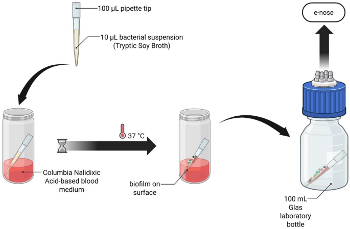
After approximately 17 h of incubation, biofilm formation was observed on pipette tips, and the structures were visually detectable across experimental conditions. In total, 56 samples were included in the analysis, bacterial cultures derived from the four pathogens, as well as control samples. Initial data-driven analysis was performed on the complete dataset including the sensor signals for all bacterial samples before conducting subgroup-specific analyses. We used cross-validation to evaluate the classification performance across measurement days. When considering the complete dataset, despite hyperparameter optimization, the maximum classification performance was below 60% across all models. Hierarchical correlation clustering did not consistently improve results, and the choice of normalization as well as the method used to aggregate cluster values varied across models. These observations highlight that optimal preprocessing strategies depend on both the classifier and the specific characteristics of the dataset. The final parameter sets and methods are provided in Supplementary Notes of the Supplementary Materials. The confusion matrix of the two best-performing models revealed frequent confusion between the species E. faecium with the control samples (see Supplementary Materials Table S2 and S3). This was likewise the case for the remaining classification models. To investigate whether feature stability, suboptimal classifier performance or biological reasons played a role in this effect, we analyzed the feature sets selected with the method described ‘Materials and Methods’ for each cross-validation training split.
Features were selected based on F-scores, prioritizing variables with stronger systematic effects and therefore with high inter-class differences and low within-class variability51. Feature selection varied across cross-validation folds, with only about 20% consistently selected. However, many fold-specific features were strongly correlated, indicating pronounced multicollinearity within the feature space. This suggests that different feature subsets reflect interchangeable representations rather than fundamentally distinct discriminative patterns, likely driven by small stochastic differences in the training data.
As shown in Fig. 3a for the first fold (i.e., first and second day as training data), the substantial overlap of confidence intervals between control samples and E. faecium across the top-ranked features indicates limited discriminative power. Because the top 20 features were selected separately for each pairwise class comparison according to their F-scores, the number of displayed features differ between Fig. 3a and b. Figure 3a shows that the test samples deviate markedly from these intervals, pointing to variability effects that mask underlying separation. Together, these observations suggest that the underlying signals may already exhibit considerable similarity between these classes, potentially contributing to the limited classification performance. In contrast, Fig. 3b reveals minimal overlap of confidence intervals between control samples and P. aeruginosa for many features, indicating distinct volatile signatures detectable by the sensor system. This is consistent with studies describing a broader range of species-specific metabolites for P. aeruginosa compared to S. aureus or E. faecalis26. For S. epidermidis, some features also show separation from controls, although less consistently. Taken together, these findings provide initial evidence that P. aeruginosa, and to a lesser extent S. epidermidis, may be distinguishable even based on single features, whereas the pronounced overlap observed for E. faecium suggests that reduced separability may originate from similarities in the underlying signal space rather than solely from limitations of the applied models.
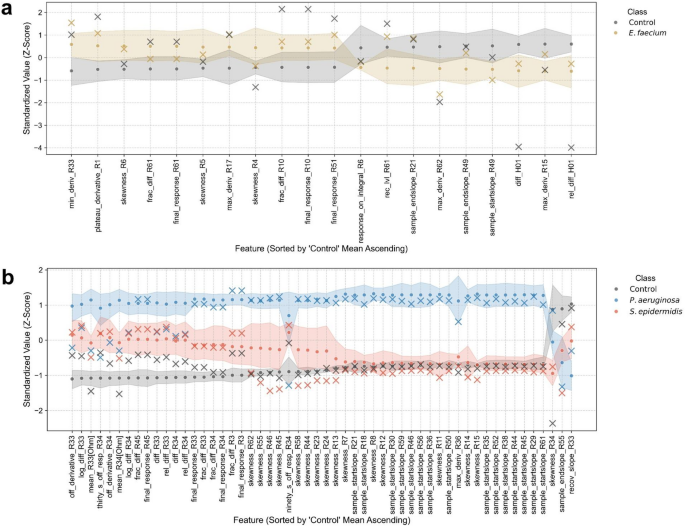
Line plot of the selected features with the highest scores. Points represent mean values over the training days, while crosses indicate mean values of the test day. Shaded areas represent the 99.5% confidence interval, calculated using the standard error of mean. The first two days were used as training set and the third day as test set (i.e., fold 1). For E. faecium and control samples (a) the confidence intervals show overlaps and the test samples lie outside the intervals of the respective class. For P. aeruginosa, S. epidermidis and control samples (b), many features exhibiting non-overlapping intervals.
Separating class overlaps from algorithmic bias
To further investigate the influence of E. faecium samples on the model performance, we removed this bacterial species from the dataset and created a new subset. With this reduced classification setting, the performance of the classifiers increased. These findings indicate that E. faecium is a critical species affecting classification performance, with all models consistently struggling to discriminate between the control samples and the E. faecium samples. This is further reflected in the recall values of the models for E. faecium and the control class. Models showing higher recall for E. faecium, such as kNN (0.67) simultaneously exhibited markedly reduced recall for the control class (0.08).
Literature indicates that E. faecium, compared to other microorganisms investigated in the respective studies, often produces fewer and more variable VOCs in lower quantity, influenced by strain differences and growth conditions, including nutrient composition52. For example, diacetyl, to which our sensors are very sensitive53, occurs in some conditions only at low levels in E. faecium profiles. In general, it has been demonstrated that VOC production varies considerably between strains, genomic variations and depends strongly on nutrient composition, with diacetyl being built in markedly different quantities under different conditions26,54. Consequently, key discriminatory volatiles may have been present only at low concentrations in our experimental setting, limiting their detectability by the sensor array. In contrast, P. aeruginosa generates a broader, more distinctive VOC spectrum, facilitating classification26. These factors likely explain the limited separability of E. faecium observed in our study, consistent with previous reports that only a small fraction of bacterial volatiles is uniquely produced by only one species26.
Examination of the confusion matrix also revealed that misclassifications predominantly involved confusion between S. epidermidis and S. aureus. As discussed later, this pattern reflects non-robust and variable sensor responses, which may have obscured subtle differences between these bacterial cultures and reduced classification stability. After excluding E. faecium and S. aureus, the classifiers were retrained on a reduced subset. A substantial improvement in accuracy and class assignment was observed, reaching a maximum accuracy of 100% (Tabl. 1). The confusion matrix of the kNN-classifier and Random Forest are given in Supplementary Materials Table S4 and S5. This pronounced performance gain on the reduced subset underscores that these two classes that were left out systematically challenged the models. As shown in the following, this is likely attributable to biological or sensor array constraints rather than algorithmic constraints.
Classification performance varied substantially across folds. Except for SVM, all classifiers achieved 100% accuracy in at least one fold, indicating that good separation was possible in some training-test splits. However, kNN accuracy ranged from 66.7% (fold 3) to 100% (folds 1 and 2), illustrating the impact of sampling variability on performance estimates. It will become clearer later why this is the case.
Within the context of previously published work on e-nose-based bacterial differentiation, our results partly align but differ markedly in the investigated model system. Sun et al. analyzed planktonic E. coli, S. aureus, and P. aeruginosa using a 34-sensor array reporting accuracies up to 96.15%55. Dutta & Dutta achieved up to 100% accuracy for planktonic E. coli, P. aeruginosa, and S. aureus56. Dias et al. reported an overall accuracy of 90% for planktonic E. faecalis, S. aureus, E. coli, and P. aeruginosa, while Suarez-Cuartin et al. achieved up to 89.2% accuracy in distinguishing P. aeruginosa from other pathogens in breath samples57,58. These examples illustrate that classification performance strongly depends not only on the applied sensor system and data analysis approach, but also on the experimental conditions, including cultivation and measurement settings. Nevertheless, in comparison with these studies, our findings demonstrate that discrimination remains feasible even under the more complex conditions of biofilm formation in blood.
The number and composition of sensors contributing to predictions varied across folds. For instance, in the decision tree classifier trained on fold 1 for the three-class classification problem, clustering reduced the feature space to five dimensions, combining multiple sensors (i.e., two aggregated clusters and three individual features). Cluster 1 contained 31 features and cluster 2 included 20 features, corresponding to a total of 30 different sensors. The two most informative clusters, defined as those with the highest Shapley values, were used for two-dimensional visualization.
The classes S. epidermidis, P. aeruginosa and control form well-defined and separable clusters in this space, indicating the presence of an underlying decision function that allows robust class discrimination, as illustrated in Fig. 4a for the first fold (i.e., the third day was used as test day). This demonstrates that a reduction to two dimensions is possible while retaining the most important discriminative information. One can observe that the test samples lie well within the clusters and are consistently classified correctly.
The observed clustering aligns with the findings of Fitzgerald et al., who reported that the VOC profile of S. epidermidis was less complex than that of the other species, containing fewer compounds and clustering closer to culture medium. Further, S. epidermidis clustered near S. aureus in our case, which is consistent with the knowledge of shared key metabolic byproducts. These metabolites are produced by both species, albeit in different quantities and intensities33. Overall, these findings indicate that VOC-based separation of these two bacterial species from control samples is feasible when grown in a biofilm-promoting environment.
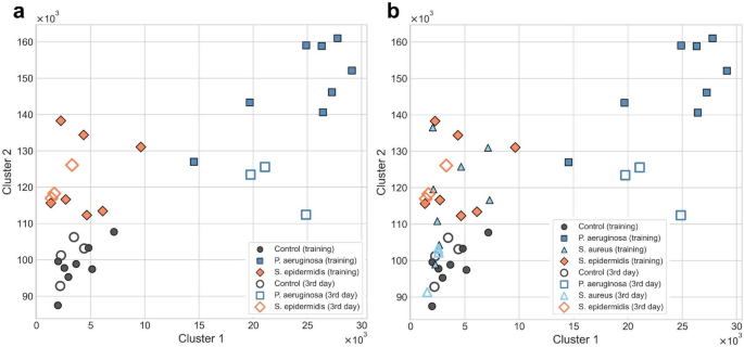
Scatter plots of bacterial samples for the first fold. Solid symbols represent training data, while unfilled symbols indicate test data points. S. aureus exhibits a wide scattering and overlaps with the control or S. epidermidis class, depending on the measurement day. A clear separation of P. aeruginosa, S. epidermidis and control can be observed (a). S. aureus scatters more and lies within the control class and S. epidermidis class (b).
In the two-dimensional representation, it becomes also evident that the species S. aureus lead to markedly different sensor-responses across days. On the first two measurement days, its responses closely resembled those of S. epidermidis, whereas on the final day they appeared more similar to the control samples in this features space, as shown in Fig. 4b. This finding is also consistent with literature and likewise shows that S. aureus has a markedly different VOC signature than P. aeruginosa32,34.
Pairwise comparison of feature means among P. aeruginosa, S. epidermidis, and Control revealed multiple statistically significant differences. Non-parametric permutation tests with 5,000 permutations and α = 0.05 were used. This approach involves random permutations of group labels of the observed data with recomputed statistics to draw statistical inference, especially valuable when only few independent observations are available59. The difference between the means was used as test statistic, and p-values were corrected for multiple comparison using the Benjamini-Hochberg procedure. After correction, 79 features differed significantly between P. aeruginosa and S. epidermidis, 31 features between S. epidermidis and Control, and 87 features between P. aeruginosa and the Control group. Effect sizes were large (Hedge’s g > 1 for 98%, and > 2 for 78% for the comparisons), and 184 of 197 significant results had corrected p-values below 0.01, indicating robust group separation. All p-values and results are given in Supplementary Table S6.
To investigate the general feasibility of discriminating samples containing bacterial growth from control samples, the task was reformulated as a binary classification problem: all bacterial samples formed one class, retrained against control samples. At this point, it should be noted that E. faecium did not provide any sensor responses that differed from the control and could not be distinguished. Therefore, we considered this task without including E. faecium. Results (Table 2) show the SVM achieved 95% accuracy, with precision 1.00 for controls and recall 0.97 for biofilms, indicating nearly all bacterial samples were correctly detected, thereby avoiding costly false negatives. Reduced recall for controls reflects their underrepresentation, highlighting that even a few misclassifications strongly affect performance metrics. Increasing control samples in future studies is expected to improve stability and reliability of these estimates. Although the overall accuracy was identical for the kNN and decision tree classifiers, differences were observed in the performance across individual folds. The kNN classifier showed a narrower accuracy range (92.3% to 93.8%), whereas the decision tree exhibited markedly greater variability, with accuracies ranging from 84.6% to 100.0%. This suggests that the kNN model produced more consistent results across different training-test splits. The Receiver Operating Characteristic curves of every classifier and fold are given in Fig. S3 of the Supplementary Materials.
It is further important to note that the overall performance is strongly affected by a single fold. Decrease of performance for some folds reflects pronounced variability between folds and thereby a lower overall cross-validation performance. In strongly imbalanced binary datasets, many commonly reported metrics can be misleading and may overestimate the model performance. As an alternative, the Matthews correlation coefficient (MCC) provides a more informative measure, as it only yields high values when the classification model performs well on both positive and negative samples, taking into account the relative proportions of the classes60. We calculated the MCC using all correct and incorrect predictions across folds, offering a fair overview of overall classification performance. For the decision tree and SVM, we obtained an MCC of approximately 0.83 and 0.89, respectively. Overall, the presented binary classification task excluding E. faecium represents a simplified best-case scenario to assess the discriminative potential of the sensor-based approach. For clinical applicability, future work must extend this to include all relevant pathogens and evaluate multi-class classification performance under complex and realistic conditions with clinical isolates.
Consideration of correlations within clusters
Out of the 62 gas sensors, we identified 11 sensors as particularly relevant for the three-class classification task. These sensors were selected in every fold. Notably, this set of chosen sensors includes several neighboring sensors, which in our e-nose system tend to be correlated and exhibit more similar baseline resistance values. Examining for example the two most relevant clusters in fold 1, cluster 2 shows stronger internal correlations than cluster 1. This difference primarily arises from the composition of the clusters: cluster 2 contains only four sensors but multiple features derived from each, whereas cluster 1 comprises 27 sensors, most of which contribute only a single feature. As a result, the features in cluster 2 are inherently more correlated. For each cluster, the feature values were condensed into one value and used as input for the models, reducing the effect of this initial multicollinearity. Using clusters of neighboring sensors could also offer a key advantage: if an individual sensor fails or produces ‘abnormal’ responses, its influence on predictions could be mitigated.
Quantifying sensor influence in model decision-making
To interpret classifier decisions and identify the most informative sensors, we performed a SHAP analysis. These values quantify the impact of each feature by considering its contribution across all possible combinations of features, providing a measure of feature importance42. By linking the important features then back to their corresponding sensors, we visualized representative sensor response curves to illustrate characteristic patterns captured by the models.
Based on the mean absolute Shapley values for the decision tree classifier in the first fold of the three-class problem, the classification decisions were exclusively driven by two clusters. Cluster 2 did not contribute to the predictions of P. aeruginosa samples, but showed the same contributions for S. epidermidis and the control class (0.34). This suggests that the cluster captured more general dynamic behavior common to bacterial classes, rather than species-specific information. The cluster consisted exclusively of derived features from four sensors, including differences, derivatives, absolute values, and their variants. On the other hand, cluster 1 was mainly driven by features describing the initial response slope and the skewness of the signal distribution across the sample exposure and recovery phase. The skewness reflected the balance between response to sample air and subsequent regeneration behavior. This cluster showed the strongest contribution to P. aeruginosa predictions (0.44), compared to S. epidermidis (0.25) and control (0.19). This indicates that cluster 1 encodes species-related signal dynamics. Similar patterns were observed across all folds, but with variations in concrete cluster composition and contribution. Overall, cluster 1 primarily drove discrimination between the two bacterial species, whereas cluster 2 mainly separated control from bacterial samples (see also Fig. 4). Notably, species discrimination required information from a broader set of sensors, whereas control separation relied on a smaller subset.
In contrast to the decision tree classifier, the kNN model did not use clustered features (see Fig. S4 in Supplementary Materials for Shapley value summary plot). The majority of the features included skewness and sample start slopes of single sensors, suggesting that early dynamic signal behavior and recovery characteristics also played a key role for this model. The distribution of the Shapley values across the three classes indicates that while some features contributed to predictions of all classes, others showed more class-specific importance. Notably, only three features deemed important by the kNN classifier were not selected by the decision tree. This strong agreement shows that both classifiers relied on similar sensor information, indicating that these sensors and features captured genuinely discriminative information rather than being selected by chance.
The SHAP values from the decision tree were mapped back from the clusters to individual sensors using weighted attributions. The SHAP value for each cluster was distributed equally among all features within this cluster. After summing up the values for different features of the same sensor within the clusters, we assigned one final value to the sensors. Figure 5 presents these aggregated Shapley values for the decision tree, providing an indication of sensor relevance across cross-validation folds. It should be noted that, due to the summation of the values, these no longer retain their original interpretability. Nevertheless, this metric allows a comparative assessment of which sensors consistently exhibited higher contributions. Two sensors were particularly important for the predictions: sensors 33 and 34. These sensors showed by far the highest values, whereas the remaining sensors exhibited markedly lower contributions. Additionally, several sensors had similar aggregated Shapley values, indicating comparable relevance.
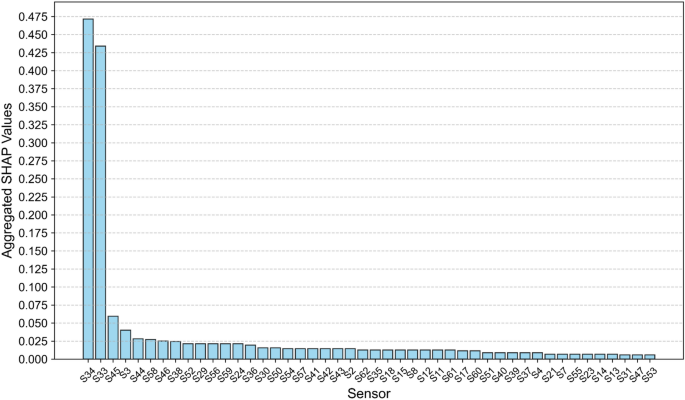
Aggregated Shapley values for each sensor that was used for prediction in at least one fold by the decision tree.
We further analyzed which features of the response curves (i.e., mean, skewness, recovery slope etc.) of these two sensors contributed most to the model’s decision. For sensor 33 and 34, the decision tree relied on steady-state as well as transient features (i.e., differences, means, derivatives and slopes). Visual inspection of the raw sensor response curves for two different days confirmed these findings (Fig. 6a and b). In particular, the response curves of these two sensors exhibited species-specific shapes, with pronounced differences in the features identified as most relevant by the models. Nevertheless, it is also evident that for S. epidermidis, the sensor response shows a varying curve shape. The agreement between model-based relevance and visually identifiable sensor response patterns demonstrates that the workflow provides a transparent and interpretable approach, leading to classification models whose decisions can be meaningfully related to underlying sensor behavior. Further, this supports the conclusion that the discrimination of bacterial cultures that can contain both planktonic and biofilm-associated cells is indeed driven by differently shaped response curves of the sensors. A visualization of these important features is given in Fig. S2 in the Supplementary Materials.
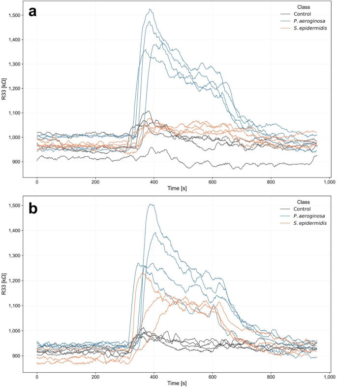
Resistance curves for every sample measurement of control, P. aeruginosa, and S. epidermidis for sensor 33 and the first (a) and second (b) measurement day. The different biofilm samples induce different sensor responses. The sensor responses were smoothed using a rolling mean with window size of 10.
This also shows that relevant information for this classification task is not confined to steady-state features, such as signal differences, but is also captured by transient characteristics, including slopes and derivatives. As reported in literature, such dynamic features can provide complementary and important discriminative information, highlighting their importance for the analysis27. It is clear that the plateau resistance values were partly not robust, but the slopes differed markedly, revealing a pronounced distinction between P. aeruginosa and the other classes.
Visual inspection of the raw sensor data also indicated substantial similarity between control measurements and E. faecium samples, with no consistent characteristic differences. This is exemplified in Fig. 7a and b for the first and second measurement day and sensor 12, which was ranked highest during feature selection. This suggests that even the sensor that was assumed as being most informative captured limited discriminative information for this comparison. It also becomes evident that the sensor responses are highly heterogeneous and vary both between and within days. As a result, the response curves lack consistent shapes and cannot be described by robust features that generalize across days.
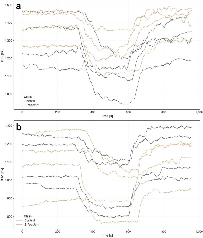
Resistance curves for every sample measurement of control and E. faecium for sensor 12 and the first (a) and second (b) measurements day. The different biofilm samples induce similar sensor responses. The sensor responses were smoothed using a rolling mean with window size of 10.
Limitations and outlook
Different limitations must be considered when interpreting these findings. First, the presented study employed a modified Lubbock chronic wound pathogenic biofilm model to investigate biofilm formation under controlled conditions. While the model reflects clinically relevant conditions such as shear stress and polymer-based surface, it remains a simplified in vitro system that cannot fully replicate the complexity of chronic wound environments. Aspects like host immune responses, spatial variability, and dynamic nutrient gradients should be kept in mind. The use of polypropylene tips as an adhesion surface offers a clinically relevant approximation of biofilm formation on polymer-based medical materials. Nevertheless, real clinical materials exhibit a wider range of surface chemistries, geometries, and aging effects, which may influence bacterial attachment and biofilm maturation. Despite these limitations, the wound model offers a controlled and reproducible method to study both planktonic and biofilm-related VOCs. Based on our study, the next step could also include measuring planktonic controls to analyze the difference between volatiles emitted from the biofilm and from planktonic cells under similar growth conditions. Besides these points, the sample size was limited, restricting the robustness of statistical estimates and possibly underestimation of classification performance. On the other hand, we also showed the presence of sample variability, which must be considered to avoid misconclusions about classifier performance. Second, the pronounced day-to-day variability influenced sensor responses and model performance, underscoring the sensitivity of gas sensor measurements to temporal and experimental conditions. In particular, S. aureus samples exhibited a broad spread across days, which had an impact on robust classification and suggests substantial variability in volatile emission patterns under the tested conditions. Although no formal drift analysis was performed, measurements were conducted across multiple experimental days, capturing day-to-day variability and thereby reflecting the practical influence of short-term drift. Nevertheless, this does not allow for a quantitative assessment of long-term sensor stability or systematic signal drift, which may affect measurements in prolonged or clinical use. Future work should therefore focus on characterizing isolated sensor drift over extended time period and evaluating calibration and correction strategies to ensure robustness in longitudinal and clinical applications. Such approaches would be essential to improve the reliability and translational potential of the sensing system, particularly in scenarios requiring repeated measurements. As this study focused on the general feasibility and exploration of differentiating biofilm-forming species in blood, sensor drift could not be isolated from biological variability, which is a prerequisite for systematically comparing correction methods. An up-to-date review of drift compensation algorithms for gas sensor arrays is provided by Li et al.61. The focus of this review lies on more advanced methods, including deep learning and transfer learning, reflecting the ongoing development of drift correction methodologies in this field. Together, these factors highlight the need for larger datasets with repeated measurements across an extended time period to reliably assess generalizability and biological variability.
A limitation of this study is that biofilm formation was not directly validated using established biofilm characterization methods such as crystal violet staining, microscopy, or viable cell quantification. Consequently, the findings should be interpreted as evidence of bacterial growth under biofilm-promoting conditions rather than detailed characterization of biofilm structure and maturity. Future studies should thus include quantitative biofilm characterization methods to better understand how biofilm structure and biomass relate to VOC signature variability and sensor-based classification performance. Future work may further incorporate GC-MS to validate e-nose signatures and link individual VOCs and metabolites to underlying sensor response patterns. This would support targeted discovery of candidate biomarkers62,63,64. Chen et al. used headspace solid-phase microextraction coupled with GC-MS to differentiate pathogenic species and to assign specific biomarkers, such as 3-methylbutanal and 3-methylbutanoic acid for S. aureus63. Boots et al. similarly demonstrated that headspace GC-MS reliably identifies microorganisms from their VOC profiles62. Further, metabolites originating from biofilms of P. aeruginosa, like 1-undecene and 2-undecanone, could be detected in concentrations in the low nanomolar range using a GC-MS based method64. As GC-MS studies in literature demonstrated that growth medium and incubation temperature determine the emitted VOC spectrum, these measurements would allow to interpret the day-to-day and species-dependent variability observed in our blood-based environment37. This could also resolve structurally overlapping profiles, particularly for E. faecium and highly variable S. aureus, and guiding biomarker selection as well as sensor array improvements.
As demonstrated by Bean et al. for P. aeruginosa, clinical isolates can exhibit substantial variability in their volatile profiles, with certain compounds consistently detected across all isolates, while others appear to be isolate-specific65. Their findings suggest the existence of a core volatilome shared among strains, alongside additional volatiles that have not previously been associated with this species. This highlights the importance of considering strain-level heterogeneity with real clinical isolates for future studies to better characterize variability in VOC patterns.
Despite the limitations of this study, the results provide initial evidence that discrimination of certain bacterial species is feasible even under clinically relevant conditions, including biofilm formation and the presence of blood. These findings also offer an indication of the potential of e-noses for biofilm identification.