Characterizing the correlations that are generated in network scenarios is a notably hard problem. For some networks, there exist simple necessary conditions for correlations to be compatible: when two parties share no causal history, their joint distribution factorizes. This is the case, for instance, of parties A1 and A6 in Fig. 1(b–ii) and (b-iii), or between the extremal parties in the entanglement-swapping network13. However, there exist networks where no such factorizations appear. The simplest example is the triangle network, obtained from the entanglement-swapping network by adding a new source connecting the extremal parties. This network, being the simplest one where explicit factorizations fail to characterize it, has been subject to intense study15,32,54,55,56,57.
In these cases without explicit factorizations, one can derive necessary conditions for correlations compatible with a network by means of inflation52,58. Briefly, inflation allows to derive compatibility constraints by imagining that multiple copies of the sources distributing physical systems and of the measurement devices held by the parties are available, and analyzing the correlations that are obtained when connecting these copies. The network structure is reflected in symmetries in the correlations on the new, inflated networks, which are much simpler to enforce and analyze (see the Methods). Indeed, many of such constraints are now present in the literature, mostly in the form of Bell-like inequalities15,54,57. The inequalities provided by inflation methods are polynomial, i.e. of the form
$$\sum _{n}\sum _{\begin{array}{c}{\vec{a}}_{1}\ldots {\vec{a}}_{n}\\ {\vec{x}}_{1}\ldots {\vec{x}}_{n}\end{array}}{c}_{{\vec{a}}_{1},\ldots ,{\vec{a}}_{n},{\vec{x}}_{1},\ldots ,{\vec{x}}_{n}}p({\vec{a}}_{1}| {\vec{x}}_{1})\cdots p({\vec{a}}_{n}| {\vec{x}}_{n})\ge 0,$$
(1)
where \({c}_{{\vec{a}}_{1},\ldots ,{\vec{a}}_{n},{\vec{x}}_{1},\ldots ,{\vec{x}}_{n}}\) are real coefficients, each \({\vec{a}}_{i}\) is a vector of outputs obtained by all parties, and \({\vec{x}}_{i}\) is the vector of corresponding inputs. These inequalities are derived naturally from the separating hyperplanes that appear when solving the linear or semidefinite programs associated to, respectively, classical58 and quantum52 inflation problems in any network. Finding for some \(p(\vec{a}| \vec{x})\) that the left-hand side evaluates to a negative quantity is a guarantee that \(p(\vec{a}| \vec{x})\) does not admit the quantum inflation used to produce the inequality. Importantly, admitting an inflation of a network is a relaxation of admitting a realization in said network. Therefore, detecting that some correlations do not admit an inflation of a network is a proof that they cannot be produced in the original network.
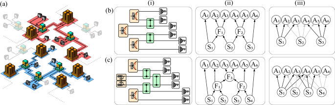
In order to illustrate the full method that we propose, let us consider the experimental realization that is used to produce six-partite Greenberger-Horne-Zeilinger (GHZ) states in ref. 41, illustrated in Fig. 1b. There, six-photon multipartite entangled states are created and distributed to six parties, A1, …, A6. Three photon-pair sources generate Bell pairs, and subsequently two fusion gates are used to obtain the final six-photon GHZ state. After the measurements, the outcome statistics follow the corresponding Born’s rule, namely
$$\begin{array}{rcl}p({a}_{1},\ldots ,{a}_{6})&=&\,\text{Tr}\,\left[{U}_{23}\otimes {U}_{45}\left({\phi }_{12}^{+}\otimes {\phi }_{34}^{+}\otimes {\phi }_{56}^{+}\right){U}_{23}^{\dagger }\otimes {U}_{45}^{\dagger }\right.\\ &&\left.\qquad \left({\Pi }_{{a}_{1}}\otimes \cdots \otimes {\Pi }_{{a}_{6}}\right)\right],\end{array}$$
(2)
where \({\phi }^{+}=\frac{1}{2}(\left\vert 00\right\rangle +\left\vert 11\right\rangle )(\left\langle 00\right\vert +\left\langle 11\right\vert )\) is the maximally entangled state, Uij is the unitary implementing the fusion gate between photons i and j, and \({\Pi }_{{a}_{i}}\) are the projectors describing the measurement operator of party Ai. One can consider distributions with inputs, p(a1, …, a6∣x1, …, x6) by using different projectors \({\Pi }_{{a}_{i}}^{{x}_{i}}\) for each measurement. For more details on the six-photon state generation, we refer to the Supplementary Materials and the original reference41.
The first step in the procedure is finding a network (i.e., a bipartite graph representation that only contains sources and parties11) that closely resembles the structure of the experiment. This network will have as many sources and outcomes as the experimental realization. Each of the sources will distribute systems to all the parties which, in the experiment, have a causal connection to it. For the setup of Fig. 1b this means that the leftmost (respectively rightmost) source will distribute systems to the three leftmost (respectively rightmost) parties, and the central source will distribute systems to the four central parties, leading to the network in Fig. 1(b–iii). Distributions that are generated in this network take the form given by the corresponding Born’s rule, i.e.,
$$p({a}_{1},\ldots ,{a}_{6})=\,\text{Tr}\,\left[\left({\rho }_{{S}_{1}}\otimes {\rho }_{{S}_{2}}\otimes {\rho }_{{S}_{3}}\right)\cdot \left({\Pi }_{{a}_{1}}\otimes \cdots \otimes {\Pi }_{{a}_{6}}\right)\right],$$
(3)
where each \({\rho }_{{S}_{i}}\) represents an arbitrary state distributed by source Si.
In order to discern whether the quantum correlations generated in the structure in Fig. 1(b–i), (b–ii) via Eq. (2) can be reproduced in the network of Fig. 1(b–iii) via Eq. (3) we will use quantum inflation52 as described in the Methods (namely, by relaxing the problem to a hierarchy of semidefinite programs that test the existence of distributions on extended scenarios with appropriate symmetries and constraints over their marginals). This implies, in particular, that we impose no restriction on the dimension of the systems distributed by the sources nor in the measurements that the parties perform on all the shares of their respective systems. We thus allow to create strong correlations between the systems in the network in Fig. 1(b–iii). Yet, we will show that these are not strong enough to reproduce the multi-photon correlations observed in Fig. 1(b–i).
In the remainder of the manuscript we focus on analyzing conditions that correlations that can be generated in the network of Fig. 1(b–iii) and how the experimental data produced in Fig. 1(b–i) (found in Ref. 41) does not meet them, showcasing the importance of the fusion gates in the realization. We must stress that our approach is fully general, not restricted to the setup in Fig. 1(b–i). In order to illustrate the generality of the approach, in the Supplementary Materials we perform an analogous analysis for the experiment carried out in ref. 40, depicted in Fig. 1c.
Witnesses of network incompatibility
When using quantum inflation, witnesses of incompatibility can be obtained in a direct manner, exploiting the fact that the compatibility of a distribution with a quantum inflation can be formulated as a semidefinite program52,59. These are optimization problems that, upon finding an incompatible distribution (recall, one for which no quantum states and measurement operators exist that reproduce it in the candidate network), provide a witness in the form of Eq. (1) that is positive for all compatible distributions and evaluates negatively at least for the incompatible one. Importantly, its evaluation to a negative quantity by any distribution is a guarantee that such distribution does not admit a realization in the candidate network.
We will obtain these witnesses for several distributions of the form of Eq. (2). Then, as a second step, we will evaluate the witnesses on the empirical data obtained in ref. 41. In order to do so, we convert the raw counts from the detectors into a probability distribution of six-photon events. The experimental setup employs measurement stages with two outputs, denoted by the transmission of a horizontally polarised photon through the polarising beam splitter or the reflection of a vertically polarised one. By normalising the number of six-photon counts (one per party) obtained in each of the possible events by the total number of six-photon counts, we obtain the empirical distributions that we will test.
Binary-input distribution
The data in ref. 41 contains counts for all the parties measuring in the X and Z bases. Therefore, it is possible to consider the two-input distribution p(a1, …, a6∣x1, …, x6), where xi = 0 corresponds to the measurement on the X basis and xi = 1 corresponds to the measurement on the Z basis. We find the resulting theoretical distribution (2), using ideal states and measurements, not to admit a realization in the network of Fig. 1(b–iii) (i.e., an expression of the form of Eq. (3)) by using its corresponding second-order inflation (depicted in Fig. 4) and, already, at the first level of the associated Navascués-Pironio-Acín (NPA) hierarchy60,61. The hierarchy is defined via sets of operators \({{\mathcal{O}}}_{n}\) that index the rows and columns of the matrix \({\Gamma }_{i,j}^{n}=\,\text{Tr}\,[\rho \cdot {O}_{i}^{\dagger }{O}_{j}]\). If a distribution admits a quantum realization, Γn is positive semidefinite for any generating set \({{\mathcal{O}}}_{n}\), and if it does not there exists at least one \({{\mathcal{O}}}_{n}\) for which Γn is negative definite. The first level of the hierarchy, which we use for analyzing the two-input distribution, is defined by the set of operators \({{\mathcal{O}}}_{1}:=\{{\mathbb{1}}\}\cup \{{A}_{p}^{i,j}\}\), leading to a matrix of size 41 × 41 in our case of interest, whose positivity can be determined in
The guarantee of incompatibility is given by the witness in Eq. S1 in the Supplementary Materials (see also the computational appendix62 for the code executed to obtain it), extracted from the problem. This witness does not only identify Eq. (2) as incompatible, but when adding white noise to the maximally entangled states, \({\phi }_{ij}^{+}\mapsto v{\phi }_{ij}^{+}+(1-v){\mathbb{1}}/4\), it identifies that the distribution is incompatible at least for v ≳ 0.6180. By increasing the accuracy of the approximations of Eq. (3) provided by inflation (see the Supplementary Materials) it is possible to guarantee incompatibility for, at least, all v ≳ 0.3887.
The evaluation on the experimental data is shown in Fig. 2. Notably, even the smallest amount of data considered, namely ~ 2900 six-photon events, representing 1% of the total amount, allows for a robust violation (namely \({{\mathcal{W}}}_{1}=-0.3420\pm 0.0466\)) well beyond the five-deviation limit. This represents an acquisition time of only 60 s per measurement basis, or equivalently, a total use of the experiment of ~1 h. In combination with the key generation results of ref. 41, this result demonstrates that it is feasible to dedicate a small amount of the data for certifying the network structure and use the rest to establish key at significantly higher rates than via concatenations of bipartite protocols.
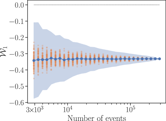
The maximum value achievable by quantum distributions generated in the network of Fig. 1(b–ii) is upper bounded by 0, so evaluating to a negative number by a given distribution is a witness that such distribution cannot be generated in Fig. 1(b–iii). In the horizontal axis we denote the amount of all datapoints, chosen at random, used for computing the witness. Error bars correspond to five standard deviations over 100 repetitions. The individual results are depicted by the orange points. The magnitude of the witness gives a notion of the distance to the set of compatible distributions, but in general it lacks of a concrete physical meaning.
We also analyze the data of ref. 40, corresponding to the network in Fig. 1c, in the Supplementary Materials. In this case, the available data allows for obtaining three binary-input distributions, corresponding to the parties performing their measurement along the bases {X−Y, X−Z, Z− Y}. We are able to obtain inequalities that witness incompatibility for all distributions for v ≳ 2−1/4. However, the differences in time spent accumulating six-photon coincidences per measurement basis (~5 min for ref. 40, totalling ~1000 six-photon events per basis, versus ~3.5 h for Fig. 1(b–i), totalling ~ 4500 six-photon events per basis), reflect themselves in the fact that the empirical distributions are not witnessed incompatible in the former case.
Tests for no-input distributions
Certifying quantum properties, such as non-locality or entanglement, in a device-independent manner necessitates of the parties performing different measurements on the shares of the states received. In contrast, it is known that constraints on the network structure are encoded even on distributions without inputs54, i.e., when the parties do not have a choice of measurement but they always measure the same operator in the received shares. One can therefore use no-input distributions to attempt at extracting guarantees of the network structure. This reduces the amount of data needed for the certification: while in the binary-input case one needs all the 212 probabilities p(a1, …, a6∣x1, …x6) for a1, …, a6, x1, …x6 ∈ {0, 1}, using no-input distributions needs only of n ⋅ 26 probabilities \({\{{p}_{k}({a}_{1},\ldots ,{a}_{6})\}}_{k = 1}^{n}\), where n is the total number of distributions tested. Therefore, in principle, one could use the techniques described earlier to give guarantees in the network structure even with fewer data. Unfortunately, this gain does not come for free. Any no-input distribution can always be simulated by a single source of shared randomness, and therefore any violation of a single inequality can always be attributed to an adversary classically correlating the parties’ outcomes. However, in the same way that the classical distribution \(p(a,b,c)=\frac{1}{2}\,\,\text{if}\,\,a=b=c\) can simulate the correlations of measurements on the Z basis performed on the state \((\left\vert 000\right\rangle +\left\vert 111\right\rangle )/\sqrt{2}\) but not those of X measurements, having a distribution being detected by several witnesses tailored for different bases gives mounting evidence of its incompatibility with a quantum network. Therefore, in the following we will extract witnesses for multiple no-input distributions, and we will evaluate each distribution in all of them to understand which distributions are easier to detect as incompatible, in the sense that they violate the largest amount of witnesses. The main results for the state created in the network in Fig. 1(b–ii) are shown in Fig. 3. There, the color code denotes the value of the witness of incompatibility of the distribution obtained by measuring the state with the operators indicating the row with the network of Fig. 1(b–iii), when evaluated in the distribution obtained by measuring the state with the operators indicating the column. More complete figures, for all possible measurement bases, can be found in the Supplementary Materials, and all the witnesses found are stored in the computational appendix62.
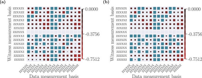
a Theoretical predictions and (b) experimental results for no-input witnesses of incompatibility with the network of Fig. 1(b–iii). The indexing of the rows and columns denotes the measurement operators that are used to generate a no-input probability distribution according to Eq. (2). Using the procedure described in the text, the distributions denoted by the rows are found to be incompatible with realizations in the network of Fig. 1(b–iii), each one producing a witness of incompatibility. Then, each witness is evaluated on all distributions denoted by the columns, producing the figures where each cell represents the evaluation of the witness obtained from the distribution in the row in the distribution in the column. The blue cells denote distributions that are not detected by a particular witness, i.e. those that evaluate to a positive value. The empty rows denote ideal distributions that are not detected to be incompatible with the inflation used. The size and the color of the red squares denote the strength of the detection for distributions witnessed to be incompatible. The complete figures with the 64 possible input combinations can be found in Figs. S1, S2 on the Supplementary Materials, and a selection of the value of the inequalities as a function of the amount of data used can be found in Fig. S3.
Since the data in ref. 41 contains statistics for all measurement choices in {X, Z}×6, we analyze all such distributions, assessing again their compatibility with the second-order quantum inflation of the network in Fig. 1(b–iii), depicted in Fig. 4. We obtain witnesses of incompatibility for a total of 40 distributions. When evaluating them on the distributions resulting from considering that the sources distribute Werner states of visibility v, these witnesses allow to detect incompatibility for visibilities ranging between 0.7808 (for the distribution corresponding to measurements XZZZZX, that establishes key between the four central parties) to 0.4094 (for the distributions corresponding to measurements ZXZZZZ, ZZXZZZ, ZZZXZZ and ZZZZXZ, that establish key between five of the six parties). Then, we evaluate the witnesses on the distributions corresponding to all measurement bases in {X, Z}×6. In Fig. 3a, b we show, respectively, the theoretical predictions for the noiseless distributions of the form of Eq. (2) and the evaluations on the empirical data, for a subset of witnesses and distributions. Analogous plots for all the witnesses and distributions can be found in Figs. S1 and S2 in the Supplementary Materials. These figures show that many distributions are witnessed as incompatible by a significant amount of inequalities, giving mounting evidence to the impossibility of generating them in the network of Fig. 1(b–iii).
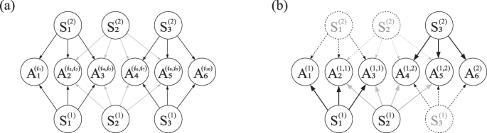
a Second-order quantum inflation of the network in Fig. 1(b–iii). There are two copies of each of the sources, and each party now has access to a different copy of the original measurement operators for each combination of states they receive. The distributions \({p}_{\inf }({\{{a}_{1}^{{i}_{1}},{a}_{2}^{{i}_{2},{i}_{3}},\ldots ,{a}_{6}^{{i}_{10}}\}}_{{i}_{1},\ldots ,{i}_{10}})\) produced in this scenario have a number of symmetries and marginals fixed by the original distribution p(a1, …, a6). The sequence of operators in (b) illustrate an assignment of indices (i1 = i2 = i4 = 1, i3 = i5 = i6 = i8 = 1, i7 = i9 = i10 = 2) that reproduces the original network, and thus the corresponding marginals must reproduce p(a1, …, a6). The fact that a \({p}_{\inf }({\{{a}_{1}^{{i}_{1}},{a}_{2}^{{i}_{2},{i}_{3}},\ldots ,{a}_{6}^{{i}_{10}}\}}_{{i}_{1},\ldots ,{i}_{10}})\) that satisfies all the necessary symmetries and marginal constraints does not exist is a proof that the premise (recall, that p(a1, …, a6) can be generated in the network of Fig. 1(b–iii)) is not true. The existence of a suitable \({p}_{\inf }({\{{a}_{1}^{{i}_{1}},{a}_{2}^{{i}_{2},{i}_{3}},\ldots ,{a}_{6}^{{i}_{10}}\}}_{{i}_{1},\ldots ,{i}_{10}})\) is a problem that can be formulated in terms of semidefinite programming59,60,61.
Remarkably, we observe a very good agreement between the theory and the experimental data. This is important given that the experimental data acquisition time per basis on a single experimental run was only 60 s and, over the course of several iterations, the data acquisition time totals ~ 3.5 hours per basis. On average, on a single run there are on the order of ~20 six-photon events. Moreover, as in the case of Fig. 2, the results are stable with regards to the amount of data used for computing the statistics. In Fig. S3 in the Supplementary Materials we illustrate this stability by plotting how a selected number of inequalities detect the incompatibility of several distributions. As we can see, even using only a fraction of the data we consistently obtain conclusive results and, when using ~2000 six-photon events, the uncertainty of the violation is below the five-sigma level. Again, we perform the equivalent analysis for the data of ref. 40, corresponding to the network in Fig. 1c, in the Supplementary Materials.