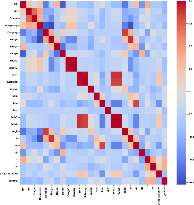
As an initial step in our data pre-processing, we employed the Z-score method to remove outliers. This procedure is essential for guaranteeing the precision and dependability of our analysis. The Z-score technique is widely recognized for its effectiveness in detecting and excluding outliers from datasets. Calculating the Z-score for every point allows us to find any outliers that significantly deviate from the rest of the dataset10. Following these steps is the process of eliminating outliers utilizing the Z-score method:
1.
Compute the Z-score for all data points11:
$$\:Z=\frac{\left(X-{\upmu\:}\right)}{{\upsigma\:}}$$
Here, X refers to each individual data point, \(\:{\upmu\:}\) indicates the dataset’s mean, and \(\:{\upsigma\:}\) indicates the standard deviation.
2.
Establish a threshold to identify outliers: A frequently used threshold value is either 2 or 3. Data points that have Z-scores higher than this threshold are classified as outliers.
3.
Remove the outliers: By eliminating these outliers, we reduce their potential impact on subsequent analysis or modeling tasks.
It should be noted that the Z-score approach supposes a Gaussian (normal) distribution of the data. Overall, the Z-score method provides a straightforward and effective approach for outlier detection and elimination, thereby improving the quality and reliability of the data analysis. The utilization of Z-score for normalization is also employed in this study. Z-score normalization is a technique employed to standardize the values of a dataset. This technique entails manipulating the data in a manner that results in a distribution with a mean equal to 0 and a standard deviation equal to 1. This is especially beneficial for comparing scores derived from disparate distributions or for optimizing the performance of machine learning algorithms.
Bayesian ridge regression (BRR)
BRR model is a strong and reliable method for analyzing regression data that combines the principles of Bayesian statistics with ridge regression. This approach offers a dynamic and adaptable framework for illustrating the relationship between separate inputs and a resulting output with continuous values12. The posterior distribution of βin this method is expressed as13,14:
$$p\left( {\beta |X,y,\alpha ,\lambda } \right) = {\text{N}}\left( {\beta |\mu ,\Sigma } \right)$$
In this equation, Σ is the covariance matrix and µrepresents the mean vector. The Bayesian method is used as follows14,15:
$$\:\mu\:={\left(\lambda\:\cdot\:{{X}^{{\prime\:}}X}^{\cdot\:}+\alpha\:\cdot\:I\right)}^{-1}\cdot\:{{X}^{{\prime\:}}y}^{\cdot\:}$$
$$\:\varSigma\:={\left(\lambda\:\cdot\:{{X}^{{\prime\:}}X}^{\cdot\:}+\alpha\:\cdot\:I\right)}^{-1}$$
Here, \(\:{X}^{{\prime\:}}y\) represents the product of the transposed input matrix and the response, \(\:{X}^{{\prime\:}}X\) signifies the result of multiplying the transpose of the matrix of input by itself, and \(\:I\)is the identity matrix14,16.
Tunable Hyperparameters for Bayesian Ridge Regression (BRR) are:
Lambda (λ): The regularization parameter, controlling the strength of regularization to prevent overfitting.
Alpha (α): Controls the variance of the coefficients’ distribution, adjusting how much they can vary.
n_iter: The maximum number of iterations for the optimization process.
Tol: The tolerance for convergence, determining when to stop optimization.
Fit Intercept: Specifies whether to calculate the intercept term for the model.
Gaussian process regression (GPR)
Given that it is both non-linear and non-parametric, GPR algorithm is a probabilistic Bayesian model that is utilized for the purpose of solving regression problems17. Unlike deterministic data-driven models that provide definite predictions, GPR offers bands of uncertainty around the predicted output values. This implies that knowledge on the variance and mean of the variables could improve the control system. By minimizing the log-marginal likelihood function, GPR effectively balances complexity and model fitting, making optimal use of the provided data18,19. The response y is denoted by \(\:f\left(x\right)\) for \(\:D=\left[\left({\varvec{x}}_{\varvec{i}},{y}_{i}\right)|i=1,\cdots\:,n\right]\), where \(\:{x}_{i}\) stands for the input matrix and \(\:{y}_{i}\)is the target value20.
$$\:y=f\left(\varvec{x}\right)$$
The characterization of a Gaussian Process (GP) is contingent on the function f(x), where random variables are delineated by implicit functions within f(x)20:
$$\:f\left(\varvec{x}\right)\sim\:{GP}\left(m\left(\varvec{x}\right),\mathbf{K}\right)$$
In the above equation, kernel covariance is denoted by K and the mean is indicated by m(x)21.
Tunable Hyperparameters for Gaussian Process Regression (GPR) are:
1.
Kernel: Specifies the covariance function, which defines the similarity between data points. Common kernels include RBF, Matern, and Rational Quadratic.
2.
Alpha: Controls the noise level in the data, allowing the model to handle noisy observations.
3.
Optimizer: Determines the method used for optimizing the kernel’s hyperparameters during training.
4.
Normalize Y: Specifies whether to normalize the target values before fitting, useful when the target has different scales.
5.
n_restarts_optimizer: Defines the number of times the optimizer is restarted to find a better set of kernel hyperparameters.
Support vector regression (SVR)
This approach seeks to optimize the discrepancy between observed and predicted values by approximating the optimal value within a specified threshold. The threshold refers to the distance separating the hyperplane from its boundary lines. SVR is a robust kernel-based regularization algorithm that improves error tolerance by allowing for a certain margin of error and adjustable error tolerance. It reduces empirical risk as well as confidence interval, regardless of input space size, while not increasing computational complexity. SVR performs well, especially with small sample sizes in high-dimensional feature spaces, offering excellent generalizability and predictive accuracy. SVR provides flexibility in defining acceptable error margins and finds a suitable hyperplane that fits the data. This process allows for the computation of a hyperplane that encapsulates the maximum number of points and establishes decision boundaries with satisfactory error margins.
Mathematically, the SVR model minimizes the following function22:
$$\:\frac{1}{2}{\left|\left|{\upbeta\:}\right|\right|}^{2}+C{\sum\:}_{i=1}^{n}\left|{{\upxi\:}}_{i}\right|$$
subject to
$$\:{\left|\left|{R}_{\text{train}}-\widehat{r}\right|\right|}_{2}^{2}\le\:\epsilon+\left|{{\upxi\:}}_{i}\right|$$
where \(\:\widehat{r}\) denotes the reconstructed reflectance calculated by \(\:\widehat{r}=X\beta\:\). Also, X stands for the matrix of output variables, \(epsilon\) denotes the margin error, \(\:{\upbeta\:}\) stands for the vector of regression model parameters, \(\:{\upxi\:}\) are the slack variables, and C is a hyperparameter defining tolerance for points outside \(epsilon\). Additionally, the kernel coefficient (\(\:{\upgamma\:}\)) determines the curvature of the decision boundary, with higher values indicating more curvature.
Tunable Hyperparameters for Support Vector Regression (SVR) are:
1.
C: Regulates the balance between attaining a minimal error on the training dataset and reducing model complexity to prevent overfitting.
2.
Kernel: Determines the method for transforming data. Common kernels include polynomial, linear, and RBF.
3.
Gamma: Indicates how far the influence of a single data point reaches, affecting the shape of the decision boundary.
4.
Epsilon (ε): Specifies the margin within which no penalty is associated with the training loss, defining the model’s tolerance to errors.
5.
Degree: Relevant for the polynomial kernel, it shows the degree of the polynomial function.
6.
Coef0: Used in polynomial and sigmoid kernels to control the influence of higher-degree terms.
Kernel ridge regression (KRR)
The method of KRR tackles the problem of determining the optimal number of independent variables in multiple regression problems. Adding more variables can result in overfitting, while reducing them can increase the variability of the model. KRR employs a function that combines the sum of squared errors with a penalty based on the count of parameters. This function estimates the parameters of a regression model23. The primal ridge regression minimization function is:
$$\:\text{minimize}\hspace{1em}{\uplambda\:}{\left|\left|w\right|\right|}^{2}+{\sum\:}_{i=1}^{\text{l}}{{\upxi\:}}_{i}^{2}$$
subject to:
$$\:{y}_{i}-\left\langle {w\cdot\:{x}_{i}} \right\rangle={{\upxi\:}}_{i},\hspace{1em}i=1,\dots\:,\text{l},$$
Here, \(\:{\uplambda\:}\) stands for the penalty term that enhances the residual sum of squares (RSS). The optimal \(\:{\uplambda\:}\)minimizes the least square error. One way to develop the Lagrangian model is by starting with this equation24:
$$\:\text{minimize}\hspace{1em}L\left(w,{\upxi\:},{\upalpha\:}\right)={\uplambda\:}{\left|\left|w\right|\right|}^{2}+{\sum\:}_{i=1}^{\text{l}}{{\upxi\:}}_{i}^{2}+{\sum\:}_{i=1}^{\text{l}}{{\upalpha\:}}_{i}\left({y}_{i}-\left\langle {w\cdot\:{x}_{i}} \right\rangle-{{\upxi\:}}_{i}\right)$$
Differentiating and imposing stationarity yields24:
$$\:w=\frac{1}{2{\uplambda\:}}{\sum\:}_{i=1}^{\text{l}}{{\upalpha\:}}_{i}{x}_{i}\hspace{1em}\text{and}\hspace{1em}{{\upxi\:}}_{i}=\frac{{{\upalpha\:}}_{i}}{2}$$
The dual problem is formulated as:
$$\:\text{maximize}\hspace{1em}W\left({\upalpha\:}\right)={\sum\:}_{i=1}^{\text{l}}{y}_{i}{{\upalpha\:}}_{i}-\frac{1}{4{\uplambda\:}}{\sum\:}_{i,j=1}^{\text{l}}{{\upalpha\:}}_{i}{{\upalpha\:}}_{j}\left\langle {{x}_{i}\cdot\:{x}_{j}} \right\rangle-\frac{1}{4}\sum\:{{\upalpha\:}}_{i}^{2}$$
which in vector form is:
$$\:W\left({\upalpha\:}\right)={y}^{{\prime\:}}{\upalpha\:}-\frac{1}{4{\uplambda\:}}{{\upalpha\:}}^{{\prime\:}}K{\upalpha\:}-\frac{1}{4}{{\upalpha\:}}^{{\prime\:}}$$
where K is the Gram matrix \(\:K_{{ij}} = \left\langle {x_{i} \cdot \:x_{j} } \right\rangle\). After applying the process of differentiation with respect to \(\:\alpha\:\) and enforcing stationarity, we obtain the following:
$$\:-\frac{1}{2{\uplambda\:}}K{\upalpha\:}-\frac{1}{2}{\upalpha\:}+y=0 \implies {\upalpha\:}=2{\uplambda\:}{\left(K+{\uplambda\:}I\right)}^{-1}y.$$
The corresponding regression function is25:
$$\:f\left(x\right)=\left\langle {w\cdot\:x} \right\rangle={y}^{{\prime\:}}{\left(K+{\uplambda\:}I\right)}^{-1}k$$
where \(\:{k}_{i}=\left\langle {{x}_{i}\cdot\:{x}_{j}} \right\rangle\). KRR simplifies Support Vector Regression.
Here’s a shortened version without values and equations:
Tunable Hyperparameters for Kernel Ridge Regression (KRR) are:
1.
Alpha: Controls the regularization strength to balance between fitting the data and preventing overfitting.
2.
Kernel: Determines the transformation of input data. Common options include linear, polynomial, and RBF kernels.
3.
Gamma: Adjusts the influence of individual data points, relevant for kernels like RBF and polynomial.
4.
Degree: Defines the degree of the polynomial kernel.
5.
Coefficient: Used in polynomial kernels to control the influence of higher-degree terms.
6.
Fit Intercept: Specifies whether to calculate the intercept term for the model.
Fireworks algorithm (FWA)
The method of FWA is a population-based optimization technique taken from the dynamics of fireworks displays. FWA mimics the explosive and attractive characteristics of fireworks to search for and determine optimal solutions within a specified search space26,27.
A population of fireworks indicates candidate solutions to the optimization task, and FWA functions by controlling this population. The process starts with random generation of first fireworks, each marked by their location and a fitness measure evaluating the quality of the solution they reflect. Explosion mechanism in the Fireworks Algorithm emulates the bursting effect of fireworks in the sky. This entails the stochastic creation of novel particles, termed sparks, in proximity to every firework. To replicate the explosion effect in this approach, FWA incorporates a Gaussian explosion amplitude formula28,29:
$$\:A=\text{exp}\left(-\frac{{r}^{2}}{2{{\upsigma\:}}^{2}}\right)$$
Following the explosion, the Fireworks Algorithm (FWA) assesses the fitness of the generated sparks, akin to the evaluation process performed by a computer scientist. Superior sparks are introduced to replace the original fireworks, resulting in an overall improvement of the population. The iterative improvement of the solutions relies heavily on this update mechanism30.
An attraction procedure is employed by FWA to point the fireworks towards the global optimum which can be obtained by presenting the subsequent equation for the amplitude of attraction28:
$$\:B=\frac{1}{\sqrt{2{\uppi\:}{\uptau\:}}}\text{exp}\left(-\frac{{r}^{2}}{2{\uptau\:}}\right)$$
where, r represents the distance between a firework and the best one, B denotes the attraction amplitude, and \(\:{\uptau\:}\)is used for tuning the strength of attraction. The attraction mechanism helps FWA to converge by guiding the fireworks towards suitable areas found during the exploration process29.
Also, the equation that determines the quantity of sparks produced by each firework, which correlates with its fitness, should also be added as:
$$\:{S}_{i}=m\times\:\left(\frac{{f}_{\text{max}}-f\left({x}_{i}\right)}{{\sum\:}_{j=1}^{n}{f}_{\text{max}}-f\left({x}_{j}\right)}\right)$$
where, \(\:{S}_{i}\) denotes the count of sparks for firework i, \(\:f\left({x}_{i}\right)\) is the fitness of firework i, \(\:{f}_{\text{max}}\) is the worst fitness value among the fireworks, and m is the spark count coefficient.
For the Gaussian mutation applied to some sparks, include the equation:
$$\:{x}^{{\prime\:}}=x+g\times\:N\left(\text{0,1}\right)$$
where g is the Gaussian mutation coefficient and N(0, 1) is a standard normal distribution.
The FWA method dynamically adjusts explosion amplitude to balance exploration and exploitation. In this method, we adjust explosion amplitude based on algorithm search performance which assures that the method initially evaluates the search space and gradually focuses on the most promising regions as optimization continues29. Figure 2 shows the optimization algorithm flowchart.
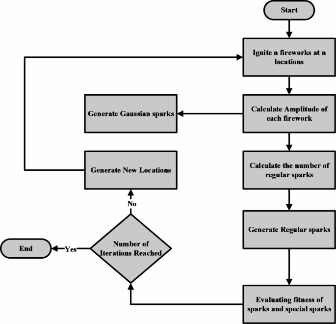
Flowchart for fireworks algorithm.
The fitness of candidate solutions in the FWA is evaluated by utilizing the mean R2 value from a 3-fold cross-validation (CV) of the model trained on the candidate solution. This approach ensures that the evaluation of the solution is both robust and generalized. In each fold of the cross-validation, the data is divided into 5 equal parts, with four parts employed to train the algorithm and one part for validating. This process is repeated five times, and the mean R2 score is computed over all the iterations, representing the solution’s effectiveness in fitting the data.
This R2 score quantifies the proportion of variance explained by the model, with values closer to 1 indicating a higher fitness. Thus, candidate solutions that yield higher mean R2 scores across the five folds are deemed to have higher fitness and are more likely to contribute to better optimization results. Also, the conditions of running FWA in this work are:
Number of Fireworks (n): 100.
Max Explosion Amplitude (A_max): 40.
Min Explosion Amplitude (A_min): 2.
Gaussian Mutation Coefficient (g): 0.0015.
Spark Count Coefficient (m): 50.
Explosion Reduction Rate (r): 0.9.
Attraction Coefficient (τ): 0.5.
Max Iterations: 100.
Performance metrics
For evaluating the predictive accuracy and effectiveness of the models used for drug solubility in polymer and gamma prediction, various performance metrics were calculated. These metrics include Mean Squared Error (MSE), Mean Absolute Error (MAE), and the Coefficient of Determination (R2 score). These metrics are essential in determining how well the model fits the data and its generalization ability.
Mean squared error (MSE)
This error metric quantifies the mean squared deviation between actual and predicted values. It imposes greater penalties on larger errors and is utilized to evaluate the precision of model predictions:
$$\:\text{MSE}=\frac{1}{n}{\sum\:}_{i=1}^{n}{\left({y}_{i}-\widehat{{y}_{i}}\right)}^{2}$$
where, \(\:{y}_{i}\) stands for the actual value, \(\:\widehat{{y}_{i}}\) signifies the predicted value, n is the total count of data points.
Mean absolute error (MAE)
This error metric calculates the average absolute deviation between the actual and predicted values. It serves as a more intuitive metric for average prediction error.
$$\:\text{MAE}=\frac{1}{n}{\sum\:}_{i=1}^{n}\left|{y}_{i}-\widehat{{y}_{i}}\right|$$
R2 score (coefficient of determination)
This measure calculates the proportion of variance in the dependent variable that can be estimated by the independent parameters in the dataset. A value closer to 1 indicates better predictive performance:
$$\:{R}^{2}=1-\frac{{\sum\:}_{i=1}^{n}{\left({y}_{i}-\widehat{{y}_{i}}\right)}^{2}}{{\sum\:}_{i=1}^{n}{\left({y}_{i}-\stackrel{-}{y}\right)}^{2}}$$
where, n stands for the count of data points. \(\:\stackrel{-}{y}\) stands for the mean of the actual values, \(\:{y}_{i}\) indicates the actual value, and \(\:\widehat{{y}_{i}}\) denotes the predicted value.
These performance metrics provide a comprehensive evaluation of model performance, ensuring accuracy and reliability in predicting drug solubility and gamma values.