#Live births, by age group and marital status of mother
#13-10-0420
tlb_nm = ’13-10-0420′
tlb_nm_pop = ’17-10-0060′
dat_raw <- get_cansim(tlb_nm) |> clean_names()
This is an ongoing trend since the 1970s and not unique to Canada
Don’t let r/Natalism see this!
Cost of living increases result in lower birthrates. It’s pretty common in every nation. Canadian cost of living has skyrocketed in the last 15 years particularly thanks to government policy to build as big a housing bubble as possible.
Canadians are struggling to find and maintain employment but the government floods the population with TFWs and international “students” so they can keep wages low.
This is pretty much exactly what I would expect although I’d be curious about absolute birth rate rather than a change in rate
I wonder if this is offset by more men having kids.
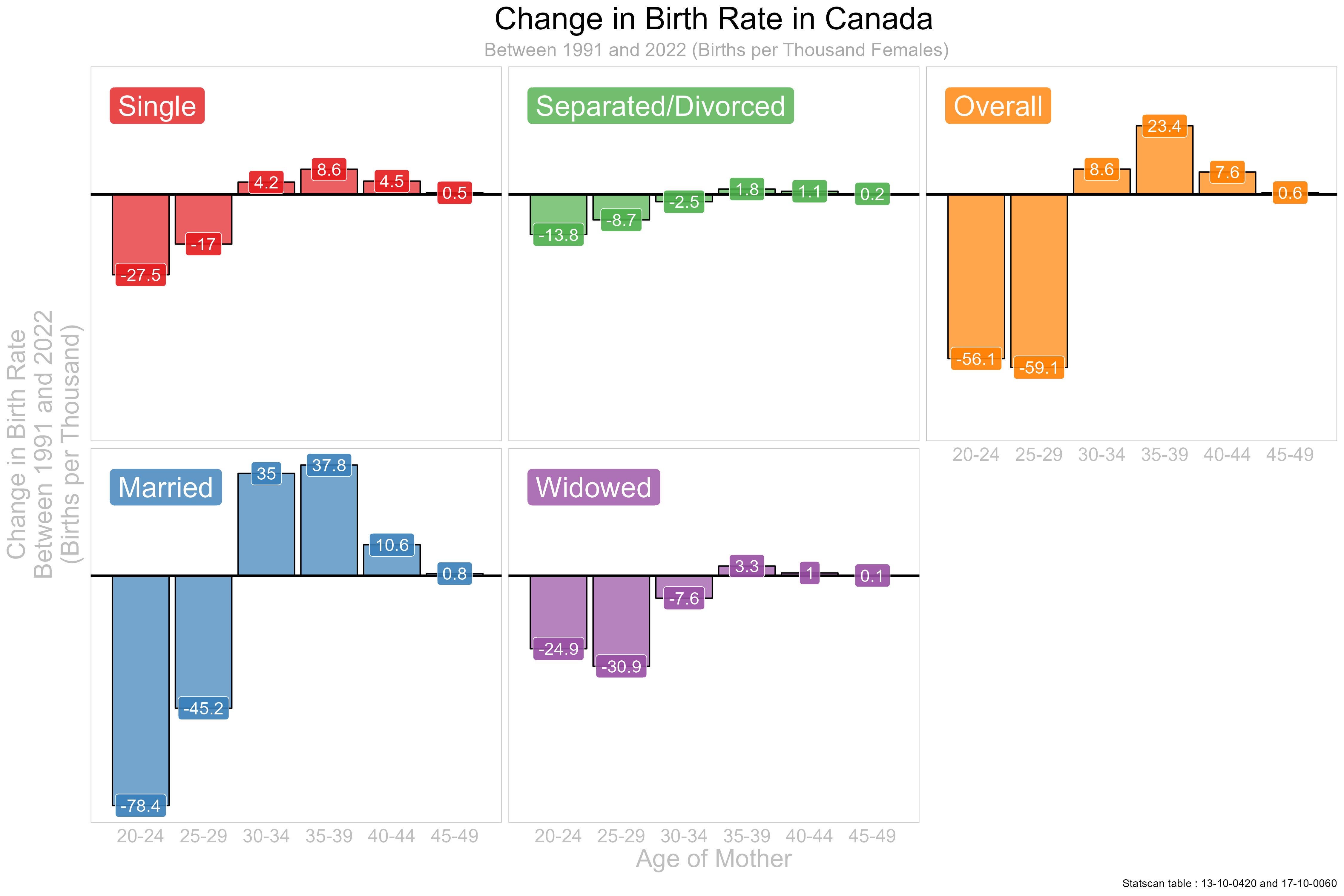
![[OC] Young Women of all Marital Statuses are Less Likely Now to Have Children in Canada.](https://www.europesays.com/wp-content/uploads/2024/12/2mm7xnpmbx5e1-1920x1024.jpeg)
7 comments
cansim tables [13-10-0420-01](https://www150.statcan.gc.ca/t1/tbl1/en/tv.action?pid=1310042001), and [17-10-0060](https://www150.statcan.gc.ca/t1/tbl1/en/tv.action?pid=1710006001), Done in R Code below :
library(scales)
library(cansim)
library(tidyverse)
library(ggplot2)
library(janitor)
library(lubridate)
library(glue)
library(feasts)
library(fpp3)
library(ggrepel)
library(magrittr)
library(RColorBrewer)
theme_set(theme_minimal())
#Live births, by age group and marital status of mother
#13-10-0420
tlb_nm = ’13-10-0420′
tlb_nm_pop = ’17-10-0060′
dat_raw <- get_cansim(tlb_nm) |> clean_names()
dat_pop_raw <- get_cansim(tlb_nm_pop) |> clean_names()
dat_pop <-
dat_pop_raw |>
filter(geo == ‘Canada’ &
sex %in% c(‘Females’) &
str_detect(age_group, ‘\s+to\s+’)) |>
mutate(yr = as.integer(ref_date)) |>
mutate(age_group = str_squish(str_remove(age_group, ‘years’))) |>
filter(str_detect(marital_status, ‘^Legal marital status,\s*’)) |>
mutate(marital_status = str_remove(marital_status, ‘^Legal marital status,\s*’)) |>
mutate(marital_status = str_remove(marital_status, ‘\s*\(.*\)$’)) |>
#filter(yr == 1991 & marital_status == ‘divorced’ & age_group == ‘0 to 14’ & sex == ‘Females’) |> View()
select(yr, marital_status, age_group, sex, value)
dat <-
dat_raw |>
filter(geo == ‘Canada, place of residence of mother’) |>
filter(marital_status_of_mother != ‘Total, marital status of mother’) |>
filter(age_of_mother != ‘Age of mother, all ages’) |>
filter(uom == ‘Number’) |>
filter(characteristics == ‘Number of live births’) |>
select(ref_date, value, age_of_mother, marital_status_of_mother) |>
mutate(
age_of_mother = str_squish(str_remove(str_remove(age_of_mother, ‘Age of mother, ‘),’years’)),
marital_status_of_mother = str_remove(marital_status_of_mother, ‘Marital status of mother, ‘),
yr = as.integer(ref_date)
) |>
mutate(marital_status_of_mother = str_remove(marital_status_of_mother, ‘\s*\(.*\)$’)) |>
#count(age_of_mother) |>
mutate(age_of_mother = recode(age_of_mother, ‘under 15’ = ‘0 to 14’ )) |>
select(-ref_date)
dat_b_rate <-
inner_join(
dat |>
rename(marital_status := marital_status_of_mother, age_group := age_of_mother , n_births = value) ,
dat_pop |>
rename(pop := value) ,
by = c(‘yr’, ‘age_group’, ‘marital_status’)
) %>%
bind_rows(
. |>
summarise(
pop = sum(pop),
n_births = sum(n_births),
.by = c(age_group, sex, yr)
) |> mutate(marital_status = ‘Overall’),
.
) |>
mutate(marital_status = if_else(marital_status %in% c(‘separated’, ‘divorced’), ‘separated/divorced’,marital_status )) |>
mutate(marital_status = factor(fct_relevel(marital_status, c(“single”, “married”, ‘separated/divorced’, “widowed”, “Overall”) ) , ordered = TRUE)) |>
summarise(pop = sum(pop , na.rm = TRUE),
n_births = sum(n_births , na.rm = TRUE),
.by = c(age_group , marital_status, sex, yr)
) |>
mutate(b_rate = n_births/(pop/1000)) |>
mutate(b_rate = ifelse(is.nan(b_rate) | is.infinite(b_rate), 0, b_rate)) |>
mutate(age_group =str_replace(age_group, ‘\s+to\s+’, ‘-‘ )) |>
filter(age_group >= ’20-24′) |>
mutate(age_group = factor(fct_relevel(age_group, sort(unique((age_group)))), ordered = TRUE)) |>
mutate(i_age_group = as.integer(age_group))
p_dat <-
dat_b_rate |>
filter(yr %in% range(yr)) |>
#filter(marital_status ==’married’ ) |>
sample_frac(size = 1) |>
mutate(yr_typ = case_when(yr == min(yr) ~ ‘min_yr’,
yr == max(yr) ~ ‘max_yr’
)
) |>
select(-yr, -n_births, -pop) |>
pivot_wider(names_from = yr_typ,
values_from = b_rate
) |>
mutate(
change_b_rate = max_yr – min_yr,
per_change_b_rate = change_b_rate/ min_yr
) #|>
#filter(marital_status != ‘Overall’)
p_mart_lbl <-
p_dat |>
mutate(change_b_rate = max(change_b_rate )*0.8 ,
i_age_group = min(i_age_group)-0.5,
) |>
summarise(change_b_rate = mean(change_b_rate),
i_age_group= mean(i_age_group),
.by = c(marital_status)
)
palette <- brewer.pal(n = length(unique(p_dat$marital_status)), name = “Set1″)
p <-
p_dat |>
ggplot(aes(y = change_b_rate, fill = marital_status )) +
geom_col(mapping = aes(x = i_age_group),alpha = 0.7, color = ‘black’) +
geom_hline(yintercept = 0, size = 1.01,
#linetype = ‘dashed’
) +
geom_label(mapping = aes(label = glue(‘{round(change_b_rate , 1)}’) , x = i_age_group), alpha = 0.9, color = ‘white’, size = 5) +
geom_label(
data = p_mart_lbl,
mapping = aes(
label = glue(‘{str_to_title(marital_status)}’),
x = i_age_group
),
size = 8,
alpha = 0.8,
color = ‘white’, hjust = 0
) +
#$geom_line() +
#geom_point() +
facet_wrap(vars(marital_status),
ncol = 3,
#scales = ‘free_y’,
dir = ‘v’
) +
labs(
y = glue(‘Change in Birth RatenBetween {paste0( range(dat_b_rate$yr), collapse =” and “)}n(Births per Thousand)’),
x = ‘Age of Mother’,
title = glue(‘Change in Birth Rate in Canada’),
subtitle = glue(‘ Between {paste0( range(dat_b_rate$yr), collapse =” and “)} (Births per Thousand Females)’),
caption = glue(‘Statscan table : {tlb_nm} and {tlb_nm_pop}’)
) +
scale_x_continuous(breaks = sort(unique(as.integer(p_dat$age_group))),
labels = (.x){
levels(p_dat$age_group)[.x]
}) +
scale_fill_manual(values = palette) +
guides(fill = ‘none’, label = ‘none’) +
theme(
axis.text.y = element_blank(),
axis.text.x = element_text(size = 15, hjust = 0.5, color = ‘grey’, angle = 0),
axis.title = element_text(size = 20, color = ‘grey’),
panel.grid = element_blank(),
panel.background = element_rect(color = ‘grey’),
strip.background = element_blank(),
strip.text = element_blank(),
plot.title = element_text(hjust = 0.5, size = 25, color = ‘black’),
plot.subtitle = element_text(hjust = 0.5, size = 15, color = ‘darkgrey’),
legend.title = element_text(color = ‘black’, size = 15),
legend.text = element_text(color = ‘black’, size = 10)
)
p
ggsave(
filename = file.path(‘images’,’change_in_fertility_rate_by_age_and_marrital_Status.jpg’),plot = p, width = 10*1.5, height = 10
)
This is an ongoing trend since the 1970s and not unique to Canada
Don’t let r/Natalism see this!
Cost of living increases result in lower birthrates. It’s pretty common in every nation. Canadian cost of living has skyrocketed in the last 15 years particularly thanks to government policy to build as big a housing bubble as possible.
Canadians are struggling to find and maintain employment but the government floods the population with TFWs and international “students” so they can keep wages low.
This is pretty much exactly what I would expect although I’d be curious about absolute birth rate rather than a change in rate
I wonder if this is offset by more men having kids.
Comments are closed.