########################
# Use this for ALL Cohorts
#
all_cohorts <-
tibble(cohort_youngest = seq(2008, 1900, by = -5),) |>
mutate(cohort_oldest = cohort_youngest – 4,
cohort = glue(‘{cohort_oldest}-{cohort_youngest}’)) |>
distinct(cohort)
########################
# Use this for Cohorts, that are in most recent data set only
cohorts <-
dat_fert_cohort |>
filter(yr == max(yr) ) |>
distinct(cohort)
2 comments
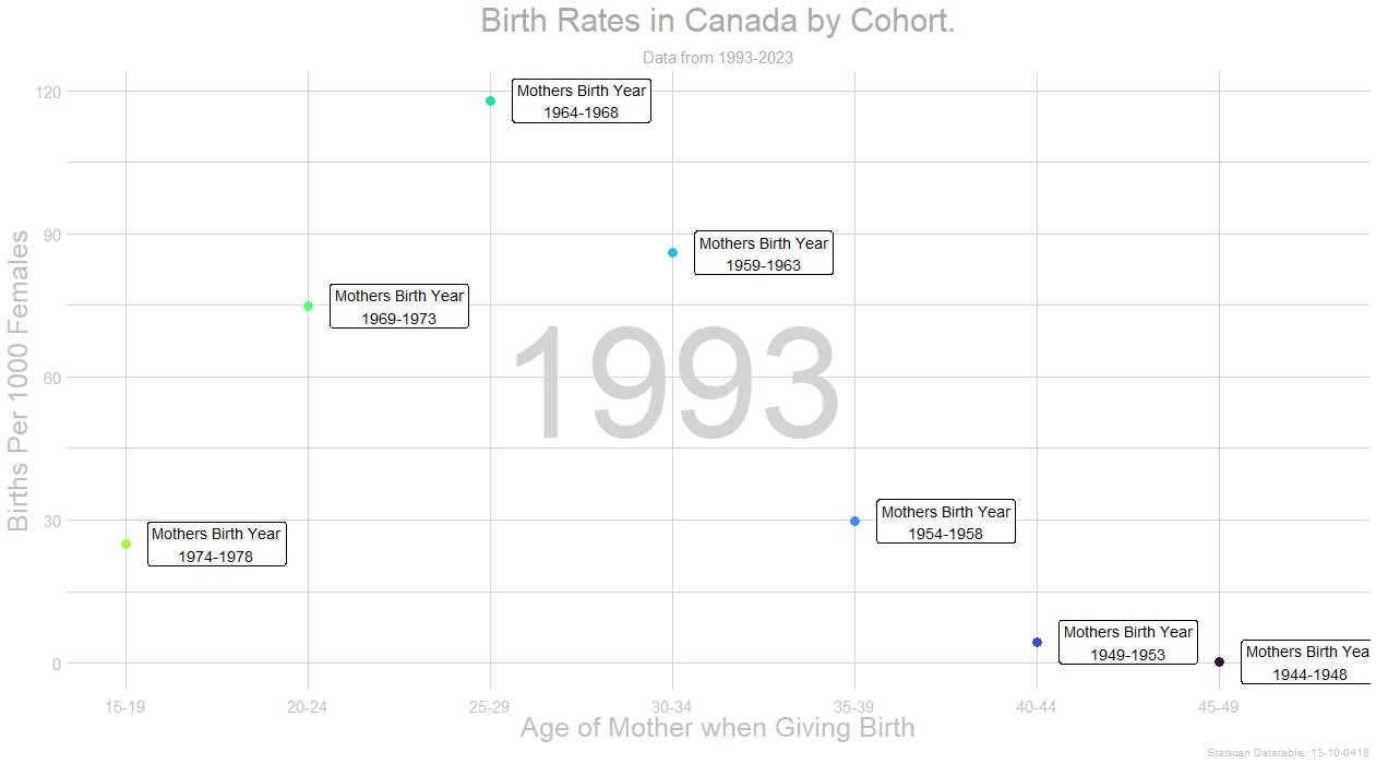
Data From [Statscan 13-10-0418](https://www150.statcan.gc.ca/t1/tbl1/en/tv.action?pid=1310041801), Code in R
library(scales)
library(cansim)
library(tidyverse)
library(ggplot2)
library(janitor)
library(lubridate)
library(glue)
library(feasts)
library(fpp3)
library(ggrepel)
library(magrittr)
library(viridis)
library(gganimate)
tlb_nm_fer <- ’13-10-0418′
fer_dat_raw <- get_cansim(tlb_nm_fer) |> clean_names()
theme_set(theme_minimal() +
theme(
axis.title = element_text(size = 15),
panel.grid = element_blank(),
plot.title = element_text(hjust = 0.5, size = 30, color = ‘darkgrey’),
plot.subtitle = element_text(hjust = 0.5, size = 15, color = ‘darkgrey’)
))
dat_fert_all <-
fer_dat_raw |>
filter(geo == ‘Canada, place of residence of mother’ &
(
str_detect(characteristics, ‘Age-specific fertility rate, females’) # |
#str_detect(characteristics, ‘Crude birth rate, live births per 1,000 population’)
)
) |>
mutate(yr = as.integer(ref_date)) |>
mutate(age_group = str_squish(str_replace(str_remove(str_remove(characteristics, ‘Age-specific fertility rate, females’), ‘years’), ‘\s+to\s+’,’-‘))) |>
#filter(yr %in% range(yr)) |>
select(yr, value, age_group)
dat_fert_cohort <-
dat_fert_all |>
mutate(age_group_min = as.integer(str_extract(age_group, ‘^([0-9]+)\-([0-9]+)$’, group = 1) ) ,
age_group_max = as.integer(str_extract(age_group, ‘^([0-9]+)\-([0-9]+)$’, group = 2) )
) |>
mutate(
cohort_youngest = yr – age_group_min ,
cohort_oldest = yr – age_group_max
) |>
mutate(
cohort = glue(‘{cohort_oldest}-{cohort_youngest}’)
) |>
mutate(age_group = factor(fct_relevel(age_group, sort(unique((age_group)))), ordered = TRUE)) |>
mutate(cohort = factor(fct_relevel(cohort, sort(unique((cohort)))), ordered = TRUE))
########################
# Use this for ALL Cohorts
#
all_cohorts <-
tibble(cohort_youngest = seq(2008, 1900, by = -5),) |>
mutate(cohort_oldest = cohort_youngest – 4,
cohort = glue(‘{cohort_oldest}-{cohort_youngest}’)) |>
distinct(cohort)
########################
# Use this for Cohorts, that are in most recent data set only
cohorts <-
dat_fert_cohort |>
filter(yr == max(yr) ) |>
distinct(cohort)
cohorts <- all_cohorts
p_dat <-
dat_fert_cohort |>
filter(cohort %in% cohorts$cohort)
p_dat_cohort_lbl <-
p_dat |>
#filter(age_group_max == max(age_group_max), .by = cohort) |>
select(cohort, age_group, value, yr)
p_dat_bg_lbl <-
p_dat |> mutate(
age_group = mean(range(as.integer(age_group))),
value = mean(range(value ))
) |>
distinct(age_group, value, yr)
yr_rng <- range(p_dat$yr)
anim <-
p_dat |>
ggplot(aes(
x = as.integer(age_group),
y = value
)) +
geom_text(
data = p_dat_bg_lbl,
mapping = aes(
label = as.character(yr),
x = as.integer(age_group),
y = value
),
inherit.aes = FALSE,
size = 50,
color = ‘lightgrey’
) +
geom_point(size = 4, aes(color = as.character(cohort))) +
geom_line(mapping = aes(
color = as.character(cohort),
group = cohort,
linetype = as.character(cohort)
),
linewidth = 1.2)+
geom_label(
data = p_dat_cohort_lbl,
mapping = aes(
label = glue(“Mothers Birth Yearn{cohort}”),
group = as.character(cohort)
),
nudge_x = 0.5,
alpha = 0.75,
hjust = 0.5,
color = ‘black’,
fill = ‘white’,
size =5
) +
scale_color_viridis_d(option = ‘H’) +
scale_fill_viridis_d(option = ‘H’) +
scale_x_continuous(breaks = sort(unique(as.integer(p_dat$age_group))),
labels = (.x){
levels(p_dat$age_group)[.x]
}) +
labs(
x = glue(‘Age of Mother when Giving Birth’),
y = glue(‘Births Per 1000 Females’),
title = ‘Birth Rates in Canada by Cohort.’,
subtitle = glue(‘Data from {yr_rng[1]}-{yr_rng[2]}’),
color = glue(‘Birth/Cohort of Mother’),
linetype = glue(‘Birth/Cohort of Mother’),
caption = glue(‘Statscan Datatable: {tlb_nm_fer}’)
) +
guides(color = ‘none’,
linetype = ‘none’,
fill = ‘none’
) +
theme(
panel.grid.major.y = element_line(color = ‘lightgrey’, linewidth = 0.01, linetype = ‘solid’),
panel.grid.minor.y = element_line(color = ‘lightgrey’, linewidth = 0.01, linetype = ‘solid’),
panel.grid.major.x = element_line(color = ‘lightgrey’, linewidth = 0.01, linetype = ‘solid’),
axis.text.x = element_text(angle = 0, size = 15, hjust = 0.5, vjust = 0, color = ‘grey’),
axis.text.y = element_text(size = 15, color = ‘grey’),
axis.title = element_text(size = 25, color = ‘grey’),
legend.title = element_text(angle = 0, size = 14, hjust = 0.5, vjust = 0, ),
plot.caption = element_text(color = ‘grey’, size = 10)
) +
transition_reveal(yr) +
enter_fade() +
exit_fade() +
ease_aes(‘linear’)
ap <-
animate(anim,
nframes = (length(unique(p_dat$yr)) * 40),
fps = 10,
end_pause = 40,
start_pause = 20,
width = 1261, # Set width in pixels
height = 700
)
ap
anim_save(file.path(‘images’, “cohort_birth_rates_by_age_and_year.gif”),
animation = ap)
Don’t forget to downvote these kinds of posts! This is not in the spirit of this sub!
Comments are closed.