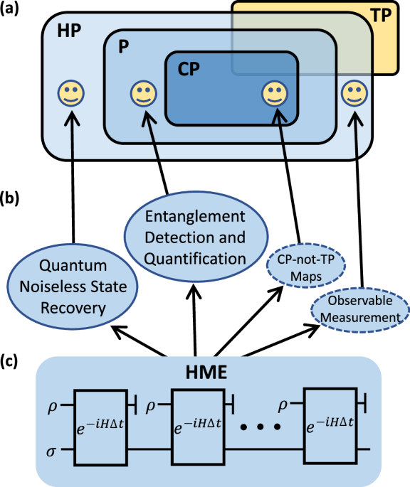
The circuit of HME is sketched in Fig. 1c. To implement the evolution of \({e}^{-i{\mathcal{N}}(\rho )t}\) on the state σ, the HME algorithm begins with preparing two quantum systems. The target state ρ will be prepared on the first system, while the second system serves as a quantum memory to keep the state on which the evolution of \({e}^{-i{\mathcal{N}}(\rho )t}\) is applied. In the beginning, the quantum memory is prepared in the initial state σ. Based on the desired accuracy, the HP map \({\mathcal{N}}\), and the total evolution time t, one determines an appropriate Hamiltonian H and a short time period Δt according to Theorem 1 and Theorem 2, respectively. Subsequently, one repeats the following steps for a total of K = t/Δt times and realizes \({e}^{-i{\mathcal{N}}(\rho )t}\) on the second system in the end:
1.
Prepare the target state ρ on the first system.
2.
Evolve the two systems jointly using e−iHΔt and discard the state on the first system.
Below, we introduce Theorem 1 to show how to choose Hamiltonian H to realize HP map \({\mathcal{N}}\).
Theorem 1
(Validation of HME). For a short time period Δt, we have
$${{\rm{Tr}}}_{1}\left({e}^{-iH\Delta t}(\rho \otimes \sigma ){e}^{iH\Delta t}\right)={e}^{-i{\mathcal{N}}(\rho )\Delta t}\sigma {e}^{i{\mathcal{N}}(\rho )\Delta t}+{\mathcal{O}}(\Delta {t}^{2}).$$
(1)
Here, \({{\rm{Tr}}}_{1}\) denotes the partial trace over the first system, \({\mathcal{N}}\) represents the target HP map, \(H={\Lambda }_{{\mathcal{N}}}^{{{\rm{T}}}_{1}}\) with \({\Lambda }_{{\mathcal{N}}}=({\mathcal{I}}\otimes {\mathcal{N}})\left\vert {\Phi }^{+}\right\rangle \left\langle {\Phi }^{+}\right\vert\) being the Choi matrix for \({\mathcal{N}}\), \(\vert {\Phi }^{+}\rangle ={\sum }_{i}\vert ii\rangle\) denotes the unnormalized maximally entangled state, and T1 represents the partial transposition operation on the first system.
This theorem can be proved using Taylor expansion and tensor network representation in Fig. 2a, b. In general, the calculation of H using \({\mathcal{N}}\) is complicated. However, in many practical applications, \({\mathcal{N}}\) has certain structures that benefit the calculation of H. An illustrative example is the partial transposition map \({e}^{-i{\rho }^{{{\rm{T}}}_{A}}t}\), where ρ is a bipartite state with two subsystems A and B. According to Theorem 1, the corresponding Hamiltonian for HME is given by \({H}_{P}={\Phi }_{A}^{+}\otimes {S}_{B}\), which has a qubit-wise tensor product form and is depicted within the red dashed box in Fig. 2c. The two blue half circles within the box represent the unnormalized maximally entangled state \({\Phi }_{A}^{+}\), while the cross of purple lines represents the SWAP operator SB. We can deduce the validity of \({{\rm{Tr}}}_{1}\left(\left[{H}_{P},\rho \otimes \sigma \right]\right)=[{\rho }^{{{\rm{T}}}_{A}},\sigma ]\) based on the connection rule of the legs.
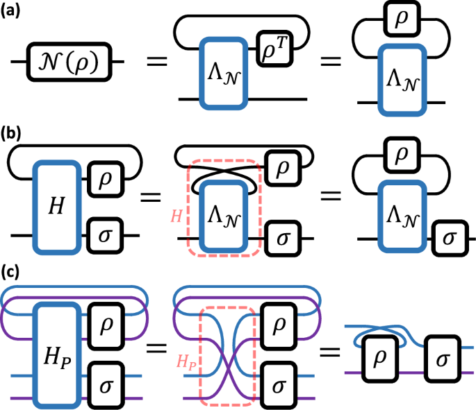
A matrix is represented using a box with left and right legs, where the left legs represent row indices and the right legs represent column indices. The connection of legs indicates the contraction between indices. In a, we illustrate the tensor network representation of the Choi matrix \({\Lambda }_{{\mathcal{N}}}\) and how it can be used to represent the action of a linear map \({\mathcal{N}}\). In b, we use the exchange of the left and right legs to represent the transposition operation. Consequently, it becomes evident that in order to ensure \({{\rm{Tr}}}_{1}[H(\rho \otimes \sigma )]={\mathcal{N}}(\rho )\sigma\), we must have \(H={\Lambda }_{{\mathcal{N}}}^{{{\rm{T}}}_{1}}\), which is highlighted by the red dashed box. In c, we graphically demonstrate the validation of \({H}_{P}={\Phi }_{A}^{+}\otimes {S}_{B}\) for realizing the evolution of \({e}^{-i{\rho }^{{{\rm{T}}}_{A}}t}\), where \({\rho }^{{{\rm{T}}}_{A}}\) is the partial transpose of ρ on system A. We use blue and purple legs to represent the indices of subsystems A and B, respectively.
According to Theorem 1, the difference between the ideal and real channels for a single step of the experiment is a second-order term. Thus the error of the whole process could be suppressed by choosing a smaller time slice Δt, or equivalently, by using more copies of ρ.
Sample complexity analysis
HME realizes the evolution of \({e}^{-i{\mathcal{N}}(\rho )t}\) by sequentially inputting the target state ρ. Thus, an essential indicator for analyzing the performance of HME is the number of copies needed for realizing the desired evolution within an error up to ϵ. We present Theorem 2 below to resolve this question.
Theorem 2
(Upper bound of sample complexity). Let \({\mathcal{N}}\) be an arbitrary HP map, the HME algorithm requires at most \({\mathcal{O}}\left({\epsilon }^{-1}{\parallel H\parallel }_{\infty }^{2}{t}^{2}\right)\) copies of sequentially inputting state ρ to ensure that \({\|{{\mathcal{Q}}_t-{\mathcal{U}}_{t}}\|}_{\diamond}\le\epsilon\) holds for arbitrary ρ. Here, \(H={\Lambda }_{{\mathcal{N}}}^{{{\rm{T}}}_{1}}\), \({{\mathcal{Q}}}_{t}={{\mathcal{Q}}}_{\Delta t}^{{\circ}{K}}\) represents the realized channel with \({{\mathcal{Q}}}_{\Delta t}(\sigma ):= {{\rm{Tr}}}_{1}\left[{e}^{-iH\Delta t}(\rho \otimes \sigma ){e}^{iH\Delta t}\right]\) and K = t/Δt, \({{\mathcal{U}}}_{t}\) is the ideal evolution channel corresponding to \({e}^{-i{\mathcal{N}}(\rho )t}\), and ∥ ⋅ ∥⋄ denotes the diamond norm.
According to the definition of the diamond norm, Theorem 2 implies that for any state \({\sigma }_{{\mathcal{K}}{\mathcal{R}}}\in {\mathcal{K}}\otimes {\mathcal{R}}\), where \({\mathcal{K}}\) is the Hilbert space on which the channels \({{\mathcal{Q}}}_{t}\) and \({{\mathcal{U}}}_{t}\) are defined, and \({\mathcal{R}}\) is a reference system with an arbitrary dimension, if the number of steps in the HME algorithm shown in Fig. 1c satisfies \(K=\Theta \left({\epsilon }^{-1}{\parallel H\parallel }_{\infty }^{2}{t}^{2}\right)\), then
$${\parallel \left({{\mathcal{U}}}_{t}-{{\mathcal{Q}}}_{t}\right)\otimes {{\mathcal{I}}}_{{\mathcal{R}}}({\sigma }_{{\mathcal{K}}{\mathcal{R}}})\parallel }_{1}\le \epsilon .$$
(2)
This implies that the states resulting from the realized and ideal evolutions are close in terms of trace distance. Consequently, when measuring the realized post-evolution state, the measurement outcomes will be close to those obtained from the ideal post-evolution state.
In practical quantum information processing tasks, the HME algorithm is often employed in conjunction with other quantum algorithms such as quantum phase estimation or Hadamard test. These algorithms typically require a controlled version of the evolution \({e}^{-i{\mathcal{N}}(\rho )t}\), as illustrated in the circuits of Fig. 4 and Fig. 5. We show that the sample complexity for exponentiating controlled \({e}^{-i{\mathcal{N}}(\rho )t}\) evolution has the same upper bound (see “Methods”).
Corollary 1
We need at most \({\mathcal{O}}\left({\epsilon }^{-1}{\parallel H\parallel }_{\infty }^{2}{t}^{2}\right)\) copies of ρ to perform \({\rm{C}}\,\text{-}\,{e}^{-i{\mathcal{N}}(\rho )t}:= \left\vert 0\right\rangle {\left\langle 0\right\vert }_{c}\otimes {\mathbb{I}}+\left\vert 1\right\rangle {\left\langle 1\right\vert }_{c}\otimes {e}^{-i{\mathcal{N}}(\rho )t}\) to precision ϵ in diamond distance, where \(H={\Lambda }_{{\mathcal{N}}}^{{{\rm{T}}}_{1}}\), and the subscript c denotes the control qubit.
Notice that \({\parallel H\parallel }_{\infty }^{2}\) might be unbounded for certain HP maps. Thus, an important problem arises: Is HME the optimal protocol for exponentiating certain HP maps? For an HP map, if the value of \({\parallel H\parallel }_{\infty }^{2}\) is large, does this mean that there exists a better algorithm, or exponentiating this HP map is fundamentally hard31,32,33,34? To finger out this problem, we first consider the most general method to exponentiate a quantum state, as shown in Fig. 3a, and use Theorem 5 to show the complexity lower bound for this general method.
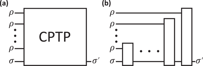
a In the most general case, joint operations are performed on multiple copies of ρ and the input state σ, which induces a channel \({\sigma }^{{\prime} }={{\mathcal{Q}}}^{\rho }(\sigma )\) that acts only on σ. b A sequential protocol relies on sequential operations acting on single-copies of ρ and the evolved state, where the black boxes represent different CPTP maps.
Combining Theorem 2 and Theorem 5, we find that the complexity upper bounds of HME can reach the lower bounds for exponentiating certain maps, as shown in Supplementary Material (see Supplementary Material for details of the algorithm). As demonstrated in Fig. 3b, HME is a special case for the general protocol. Therefore, we can conclude that for maps such as the inverse of local amplitude damping noise channel, the HME algorithm is the optimal method to realize \({e}^{-i{\mathcal{N}}(\rho )t}\). It is also worth mentioning that the analysis of the upper and lower bounds for realizing \({e}^{-i{\mathcal{N}}(\rho )t}\) also partly answers the open problem raised in ref. 35. This problem seeks to determine the sample complexity required for implementing the evolution of e−if(ρ)t for a given function f(⋅). Note that when only concentrating on expectation values, the optimal sampling overhead for simulating the HP map \({\mathcal{N}}\) is determined by \({\|{{\mathcal{N}}}\|}_{\diamond}^{2}\) using the quasi-probability decomposition method32,36. Further study is required to characterize the optimal sample complexity of simulating HP maps through exponentiation.
In practical situations, the performance of HME can be affected by various factors. For example, quantum devices may exhibit unpredictable and unavoidable noise, and the realization of the Hamiltonian evolution e−iHΔt may be inaccurate due to approximation errors in Hamiltonian simulation37,38. Besides, the input state ρ may also be affected and deviate in each step. We analyze the robustness of HME against the input state error and the Hamiltonian error in the Supplementary Material (see Supplementary Material for details of the algorithm). Similar to the sample complexity, we show that the robustness of HME is also influenced by ∥H∥∞, which could help us to find application scenarios.
Entanglement detection
Entanglement is a distinctive feature of quantum mechanics39, and the detection and quantification of entanglement is of both fundamental and practical importance40,41. A variety of protocols have been proposed for entanglement detection3. The positive map criteria, which include the partial transposition6 and reduction maps42, are considered to be among the most powerful entanglement detection criteria43. The positive map criterion states that if \({{\mathcal{P}}}_{A}\otimes {{\mathcal{I}}}_{B}(\rho )\) is not a semi-positive matrix, then the state ρ is entangled. Here, \({\mathcal{P}}\) represents the positive map being used, and A and B label the two subsystems of ρ. However, the main challenges in achieving positive map detection protocols lie in the non-CP nature of positive maps as well as the difficulty of performing spectral analysis for the exponentially large matrix \({{\mathcal{P}}}_{A}\otimes {{\mathcal{I}}}_{B}(\rho )\). These two obstacles can be overcome using the algorithms of HME and quantum phase estimation.
Combining the ability of HME to exponentiate the controlled unitary operation \({e}^{-i{{\mathcal{P}}}_{A}\otimes {{\mathcal{I}}}_{B}(\rho )t}\) and the quantum phase estimation algorithm, we propose an HME-based entanglement detection protocol, as illustrated in Fig. 4a. The measurements of the ancilla qubits directly provide information about the spectrum of \(U={e}^{-i{{\mathcal{P}}}_{A}\otimes {{\mathcal{I}}}_{B}(\rho )t}\), which is equivalent to the spectrum of \({{\mathcal{P}}}_{A}\otimes {{\mathcal{I}}}_{B}(\rho )\). If \({{\mathcal{P}}}_{A}\otimes {{\mathcal{I}}}_{B}(\rho )\) is not semi-positive, we can select σ to be a state that exhibits significant overlap with the negative subspace of \({{\mathcal{P}}}_{A}\otimes {{\mathcal{I}}}_{B}(\rho )\). Consequently, there is a significant probability of detecting the negative eigenvalues of \({{\mathcal{P}}}_{A}\otimes {{\mathcal{I}}}_{B}(\rho )\) and thus the entanglement of ρ.
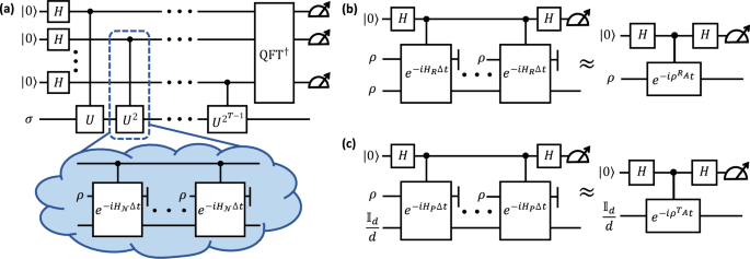
a Represents the circuit of the HME-based entanglement detection protocol, which is constructed by combining the HME and quantum phase estimation algorithms. The quantum phase estimation consists of the input state σ, T ancilla qubits, controlled unitary operations, inverse quantum Fourier transformation, and final measurements on the ancilla qubits. The controlled unitary evolutions are approximately realized by HME, where \({H}_{{\mathcal{N}}}\) is the Hamiltonian for exponentiating \({\mathcal{N}}={{\mathcal{P}}}_{A}\otimes {{\mathcal{I}}}_{B}\). b Is a special case of a where only one ancilla qubit remains, the inverse quantum Fourier transformation is reduced to the Hadamard gate, and HR is the Hamiltonian for exponentiating the partial reduction map. The evolved state and sequentially inputted states are set to the target state of the entanglement detection task. c Is the circuit for estimating entanglement negativity. Compared with b, we change the evolved state to the maximally mixed state and the Hamiltonian to HP.
This new protocol offers a systematic approach to leverage quantum resources such as quantum memory and ancilla qubits, enabling us to reduce classical repetition times and gain advantages over conventional methods. Specifically, it has been proven that if only single-copy operations are allowed, an exponential amount of resources is required for entanglement detection43, even in the case of pure states44. The following presents a typical example.
Fact 1
Consider a bipartite system with subsystem dimensions \({d}_{A}={d}_{B}=\sqrt{d}\) 44. Let ρ be a pure state, which can be either a global Haar random state ψAB or a tensor product of local Haar random pure states ψA ⊗ ψB, each with equal probabilities. If we are limited to single-copy operations and measurements on ρ, determining whether ρ is entangled requires Θ(d1/4) experiments, with a success probability of at least 2/3.
Here we employ the reduction map to demonstrate the advantage of HME in entanglement detection. The reduction map R is defined as \({\rho }^{R}={\rm{Tr}}(\rho ){{\mathbb{I}}}_{d}-\rho\), where d = dA × dB represents the dimension of the Hilbert space of ρ. The reduction criterion involves testing whether
$${\rho }^{{R}_{A}}={{\mathbb{I}}}_{{d}_{A}}\otimes {\rho }_{B}-\rho$$
(3)
is semi-positive or not, where \({\rho }_{B}={{\rm{Tr}}}_{A}(\rho )\) denotes the reduced density matrix for subsystem B. By exponentiating the partial reduction map using HME, we find that the entanglement detection task implied in Fact 1 can be solved with a constant sample complexity using the HME-based entanglement detection protocol, showing an exponential advantage compared with all single-copy entanglement detection protocols. Besides, the circuit for this task is shown in Fig. 4b, which requires only a single ancilla qubit.
Theorem 3
Let \({H}_{R}={{\mathbb{I}}}_{A}\otimes {S}_{B}-{S}_{AB}\), where \({{\mathbb{I}}}_{A}\), SB, and SAB stand for the identity operator acting on two copies of system A, SWAP operator acting on two copies of system B, and SWAP operator acting on two copies of the joint system AB, respectively. Choosing t = π, the circuit depicted in Fig. 4b requires at most \({\mathcal{O}}(1)\) copies of ρ to accomplish the task described in Fact 1 with a success probability of at least 2/3.
In addition to the constant sample complexity, the corresponding Hamiltonian \({H}_{R}={{\mathbb{I}}}_{A}\otimes {S}_{B}-{S}_{AB}\) is 2-sparse and efficiently row computable. As a result, it can be efficiently simulated45, leading to an overall gate complexity of our protocol that scales as \({\mathcal{O}}(1)\).
Entanglement quantification
Among all positive map criteria, the positive partial transposition criterion6 is of fundamental importance due to its strong detection capability46, its connection to entanglement distillation9, and its concise mathematical formulation. The positive partial transposition criterion states that if the target state ρ is separable, then the matrix \({\rho }^{{{\rm{T}}}_{A}}\) has no negative eigenvalues, where TA denotes the partial transposition map on a subsystem A. The entanglement negativity serves as an entanglement measure by quantifying the violation of the positive partial transposition criterion,
$$N(\rho )=\frac{{\parallel {\rho }^{{{\rm{T}}}_{A}}\parallel }_{1}-1}{2},$$
(4)
which equals the sum of the absolute values of all negative eigenvalues of \({\rho }^{{{\rm{T}}}_{A}}\). As a widely used quantifier for mix-state entanglement, negativity plays an indispensable role in theoretical physics8,47,48.
However, due to the non-CP nature of the transposition map and the highly nonlinear behavior of negativity, there is still no efficient protocol for unbiasedly estimating negativity. Some approaches, such as directly measuring the spectral values of \({\rho }^{{{\rm{T}}}_{A}}\)21,49, require joint operations on exponentially many copies of quantum states. Tomography-based protocols estimate negativity by reconstructing the density matrix, which requires a large sample complexity and significant classical computational resources50,51. Other attempts primarily utilize the moments of the partially transposed density matrix to infer properties of negativity10,52, rather than providing an unbiased estimation.
HME can also alleviate the difficulties in measuring negativity. Firstly, as illustrated in Fig. 2c, HME can realize the evolution of \({e}^{-i{\rho }^{{{\rm{T}}}_{A}}t}\) by setting the evolution Hamiltonian to \({H}_{P}={\Phi }_{A}^{+}\otimes {S}_{B}\). Secondly, as \({e}^{-i{\rho }^{{{\rm{T}}}_{A}}t}\) is a nonlinear function of \({\rho }^{{{\rm{T}}}_{A}}\), HME enables the measurement of certain nonlinear quantities including entanglement negativity53,54. Specifically, we can combine the HME algorithm and Hadamard test algorithm and use the circuit shown in Fig. 4c to estimate \({\rm{tr}}\,[\cos ({\rho }^{{{\rm{T}}}_{A}}t)]\) in different values of t. According to Fourier decomposition, we can use these quantities to construct an unbiased estimation of entanglement negativity. We show details of this estimation protocol in Methods.
Theorem 4
One needs an expected number of \(\widetilde{{\mathcal{O}}}\left(\log ({\delta }^{-1}){\epsilon }^{-3}{d}^{2}{d}_{A}{\parallel {\rho }^{{{\rm{T}}}_{A}}\parallel }_{1}\right)\) copies of ρ to ensure \(\left\vert \hat{N}(\rho )-N(\rho )\right\vert \le \epsilon\) with a probability of at least 1 − δ. Here, the \(\widetilde{{\mathcal{O}}}\) notation suppresses logarithmic expressions for d and ϵ, dA stands for the dimension of subsystem A.
We leave the technical proof of Theorem 4 in the Supplementary Material (see Supplementary Material for details of the algorithm). Due to the property of entanglement negativity, \({\parallel {\rho }^{{{\rm{T}}}_{A}}\parallel }_{1}={\parallel {\rho }^{{{\rm{T}}}_{B}}\parallel }_{1}\), we can always assume dA ≤ dB. As \({\parallel {\rho }^{{{\rm{T}}}_{A}}\parallel }_{1}\le {d}_{A}\), the worst case sample complexity is at most \(\widetilde{{\mathcal{O}}}\left({\epsilon }^{-3}{d}^{3}\right)\). Compared to the tomography-based negativity estimation protocol, our protocol has advantages in both quantum and classical resource consumption. Due to the fact that negativity can be exponentially large, the tomography-based protocol requires θ(ϵ−2d4) repetition times to accurately estimate negativity51. Thus, HME showcases polynomial improvement in sample complexity. Additionally, the tomography-based protocol requires performing spectral decomposition of the reconstructed density matrix, which also consumes exponential classical resources for computation and memory. Since the HME-based protocol relies on directly accessible quantities, we can save these classical resources.
Quantum noiseless state recovery
Noises in quantum circuits act as a significant obstacle to implementing quantum algorithms55,56. Researchers have dedicated significant efforts to handling quantum noises, resulting in various protocols that can be categorized into two main types: quantum error correction and mitigation. By encoding the target state into a larger Hilbert space, quantum error correction protects the target state against a large variety of errors57,58,59,60. When the physical noise rate is below a certain threshold61, quantum error correction can suppress the logical error rate to an arbitrarily small value by consuming a large number of ancilla qubits62. Quantum error mitigation4,5 focuses on a simpler task of recovering the noiseless expectation value using multiple noisy states. Some error mitigation protocols are tailored to handle specific types of noises, such as virtual distillation63,64 for incoherent errors and subspace expansion for coherent errors65. Some protocols are designed to handle general forms of noises, such as probabilistic error cancellation12,13,14, which is one of the leading error mitigation approaches. Quantum error mitigation typically requires an exponential number of experiments to accurately estimate the noiseless expectation value66,67.
Building upon HME, we propose a new protocol to handle quantum noises, which is named quantum noiseless state recovery. We consider a similar setting as quantum error mitigation where many noisy states are provided. Suppose the ideal noiseless state ψ is generated by an ideal noiseless circuit, \(\psi ={\mathcal{U}}(\left\vert 0\right\rangle \left\langle 0\right\vert )\), while the existence of noise will change it to \({\mathcal{E}}(\psi )={\mathcal{E}}\circ {\mathcal{U}}(\left\vert 0\right\rangle \left\langle 0\right\vert )\). Note that \({{\mathcal{E}}}^{-1}\) is always HP when it exists31, thus the exponentiation of \({{\mathcal{E}}}^{-1}\) becomes possible with HME. By sequentially inputting multiple copies of \({\mathcal{E}}(\psi )\) into the circuit depicted in Fig. 1c and choosing an appropriate Hamiltonian, we can approximately realize the evolution of
$${e}^{-i{{\mathcal{E}}}^{-1}\circ {\mathcal{E}}(\psi )t}={e}^{-i\psi t}$$
(5)
with arbitrary accuracy.
It is evident that e−iψt has only one nontrivial eigenvalue, e−it, with the corresponding eigenstate \(\vert \psi \rangle\). Setting t = π, a simple circuit shown in Fig. 5 can be used to prepare the noiseless state ψ and thus serves as the circuit for quantum noiseless state recovery. The correctness of our protocol is ensured by the following proposition:
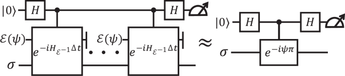
The Hamiltonian is set to be \({H}_{{{\mathcal{E}}}^{-1}}={\Lambda }_{{{\mathcal{E}}}^{-1}}^{{{\rm{T}}}_{1}}\), the partial transposition of the Choi matrix of the inverse map \({{\mathcal{E}}}^{-1}\). The evolved state σ serves as a guiding state which needs to have a high fidelity with the noiseless state ψ.
Proposition 1
When measuring the ancilla qubit in the ideal circuit depicted on the right side of Fig. 5, the outcome \(\left\vert 1\right\rangle\) occurs with a probability of \(\langle \psi \vert \sigma \vert \psi \rangle\). If the outcome \(\vert 1\rangle\) is observed, σ will evolve into the desired noiseless pure state \(\vert \psi \rangle\).
Note that in a practical situation where the noise rate is relatively small, one can choose the noisy state \({\mathcal{E}}(\psi )\) as the evolved state σ to increase the success probability. Considering the approximation error of the HME algorithm and the success rate of post-selection, we derived the performance of our noiseless state recovery protocol, shown in Theorem 6 in Methods.
Quantum noiseless state recovery faces practical challenges of requiring precise knowledge of the noise channel, the calculation of the inverse map, and efficient methods for realizing controlled Hamiltonian evolution. However, its fundamental differences from conventional error management protocols offer inspiration for alternative error management protocols and warrant a deeper understanding of its characteristics. Notably, quantum noiseless state recovery is the first protocol that can recover the noiseless quantum state without any encoding operation. Specifically, our protocol starts from states that have already been influenced by noises, like quantum error mitigation. However, what sets our protocol apart is its capacity to recover noiseless quantum states. Such ability brings advantages in various applications5, such as quantum storage and quantum communication, where noise-free states are desired. It is also crucial in practical scenarios like the Shor algorithm and quantum key distribution, where noiseless states enable obtaining single-shot measurement results instead of just expectation values. Compared to quantum error correction, our protocol requires fewer ancilla qubits and does not necessitate access to the noiseless state at the beginning. A more comprehensive comparison can be found in the Supplementary Material (see Supplementary Material for details of the algorithm).