Various definitions of negativity in the literature share a common and central dependency, namely, the partial transpose of the density matrix. In this work, we adopt the partial time-reversal transformation proposed by Shapourian et al.38,39 as the FPT.
We begin with the general partitioning of a fermionic lattice model. It is defined using annihilation (creation) operators \({c}_{j\sigma }^{({{\dagger}} )}\), which satisfy the anticommutation relations \(\{{c}_{j\sigma },{c}_{k{\sigma }^{{\prime} }}^{{{\dagger}} }\}={\delta }_{jk}{\delta }_{\sigma {\sigma }^{{\prime} }}\), where j, k = 1, …, N are the labels of the sites and \(\sigma,{\sigma }^{{\prime} }\) are the indices for internal degrees of freedom such as spin. In the following discussion, we may use a column vector \({{{\bf{c}}}}={({c}_{1,\uparrow },\ldots,{c}_{N,\uparrow },{c}_{1,\downarrow },\ldots,{c}_{N,\downarrow })}^{T}\) to compactly encapsulate all the fermionic operators. This lattice system, denoted as A, generally exists within a larger space, as illustrated in Fig. 1a. After tracing out the environment \(\bar{A}\), system A typically exists in a mixed state ρ. For example, if system A is in contact with a much larger thermal bath at temperature T, then we obtain a finite-temperature Gibbs state \(\rho={e}^{-\beta H}/{{{\rm{Tr}}}}{e}^{-\beta H}\) with β = 1/T the inverse temperature and H the Hamiltonian of the system A. Next, we further divide system A into two parties belonging to two complementary spatial regions respectively, i.e., A = A1 ∪ A2. Then the density matrix acting on Hilbert space \({{{{\mathcal{H}}}}}_{1}\otimes {{{{\mathcal{H}}}}}_{2}\) can be expanded as \(\rho={\sum }_{{A}_{1},{A}_{2},{A}_{1}^{{\prime} },{A}_{2}^{{\prime} }}{\rho }_{{A}_{1},{A}_{2};{A}_{1}^{{\prime} },{A}_{2}^{{\prime} }}\left\vert {A}_{1}\right\rangle \left\vert {A}_{2}\right\rangle \left\langle {A}_{1}^{{\prime} }\right\vert \left\langle {A}_{2}^{{\prime} }\right\vert\).
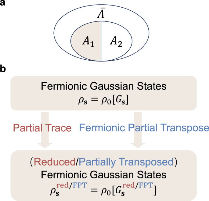
a Illustration of the general tripartite geometry. First, we trace out the environment \(\bar{A}\) to obtain the reduced density matrix ρA, and then evaluate the entanglement between subsystems by either tracing out or partially transposing A2. b The fermionic partial transpose of Gaussian states, \({\rho }_{0}[G] \sim {e}^{{{{{\bf{c}}}}}^{{{\dagger}} }\ln ({G}^{-1}-I){{{\bf{c}}}}}\), remains Gaussian. These states represent free fermions, including the auxiliary-field-dependent density matrix ρs in the DQMC framework. The reduced and partially transposed density matrices thus share a unified expression in terms of the corresponding Green’s functions. Specifically, the reduced Green’s function is \({G}_{{{{\bf{s}}}},{A}_{1}}^{{{{\rm{red}}}}}={\langle {c}_{j}{c}_{k}^{{{\dagger}} }\rangle }_{{{{\bf{s}}}}}\) for j, k ∈ A1, while the partially transposed Green’s function \({G}_{{{{\bf{s}}}},{A}_{1}}^{{{{\rm{FPT}}}}}={G}_{{{{\bf{s}}}}}^{{T}_{2}^{f}}\) is given by Eq. (3).
The FPT of density matrix ρ with respect to subsystem A2, denoted as \({\rho }^{{T}_{2}^{f}}\), exhibits a highly succinct mathematical expression in the Majorana basis38,39. Under Majorana basis, an arbitrary density operator can be expressed as a constrained superposition of products of Majorana operators, which are defined as \({\gamma }_{2j-1,\sigma }={c}_{j,\sigma }+{c}_{j,\sigma }^{{{\dagger}} }\) and \({\gamma }_{2j,\sigma }=-{{{\rm{i}}}}({c}_{j,\sigma }-{c}_{j,\sigma }^{{{\dagger}} })\). It is found that \({\rho }^{{T}_{2}^{f}}\) can be obtained by applying the following transformation to the Majorana operators associated with subsystem A2:
$${{{{\mathcal{R}}}}}_{2}^{f}({\gamma }_{j,\sigma })=\,{\mbox{i}}\,{\gamma }_{j,\sigma },\quad j\in {A}_{2}.$$
(1)
Remarkably, under this definition, the partial transpose of a Gaussian state, denoted as \({\rho }_{0} \sim {e}^{\frac{1}{4}{{{{\boldsymbol{\gamma }}}}}^{T}W{{{\boldsymbol{\gamma }}}}}\) with \({{{\boldsymbol{\gamma }}}}={({\gamma }_{1,\uparrow },\ldots,{\gamma }_{2N,\uparrow },{\gamma }_{1,\downarrow },\ldots,{\gamma }_{2N,\downarrow })}^{T}\), retains its Gaussian nature. The question then pertains to determining the explicit form of \({\rho }_{0}^{{T}_{2}^{f}}\) or \({W}^{{T}_{2}^{f}}\). To this end, it is important to emphasize that a Gaussian state ρ0 can be alternatively characterized by the Green’s function Γkl = 〈[γk, γl]〉/2, which is averaged with respect to ρ0 itself and also called covariance matrix.
This matrix is connected to the W matrix through the relation \(\tanh (-W/2)=\Gamma\), or inversely, \(W=\ln \left[{(I+\Gamma )}^{-1}(I-\Gamma )\right]\)50 (see also the Supplementary Note 3 for a proof). By employing the definition of Γ and the partial transpose in the Majorana basis (refer to Eq. (1)), the partial transpose of the covariance matrix can be formulated as
$${\Gamma }^{{T}_{2}^{f}}=\left(\begin{array}{cc}{\Gamma }^{11}&\,{\mbox{i}}\,{\Gamma }^{12}\\ \,{\mbox{i}}\,{\Gamma }^{21}&-{\Gamma }^{22}\end{array}\right),$$
(2)
where \({\Gamma }^{b{b}^{{\prime} }}\) (\(b,{b}^{{\prime} }=1,2\)) denotes the block comprising the matrix elements with rows pertaining to subsystem Ab and columns pertaining to subsystem \({A}_{{b}^{{\prime} }}\). The Gaussian state described by \({\Gamma }^{{T}_{2}^{f}}\) precisely yields \({\rho }_{0}^{{T}_{2}^{f}}\) through the relation \(\tanh (-{W}^{{T}_{2}^{f}}/2)={\Gamma }^{{T}_{2}^{f}}\), i.e., \({({\rho }_{0}[\Gamma ])}^{{T}_{2}^{f}}={\rho }_{0}[{\Gamma }^{{T}_{2}^{f}}]\) with \({\rho }_{0}[\Gamma ] \sim {e}^{{{{{\boldsymbol{\gamma }}}}}^{{T} }\ln \left[{(I+\Gamma )}^{-1}(I-\Gamma )\right]{{{\boldsymbol{\gamma }}}}}\). This elegant fact is proved using Wick’s theorem for Majorana monomials36 (see the Supplementary Note 3 for details).
The above discussion in the Majorana basis can be seamlessly transitioned to the complex fermion basis. In complex fermion basis, the Green’s function is defined as \({G}_{jk}=\langle {c}_{j}{c}_{k}^{{{\dagger}} }\rangle\), where we have abbreviated the spin indices. Its partially transposed form exhibits also a simple structure
$${G}^{{T}_{2}^{f}}=\left(\begin{array}{cc}{G}^{11}&\,{{\mbox{i}}}\,{G}^{12}\\ \,{{{\rm{i}}}}\,{G}^{21}&I-{G}^{22}\end{array}\right),$$
(3)
where the superscripts of the blocks \({G}^{b{b}^{{\prime} }}\) indicate the subsystems, akin to the notation of \({\Gamma }^{b{b}^{{\prime} }}\) established earlier. Similar to the Majorana basis, the above Green’s function delineates another Gaussian state which is exactly the partial transpose of the original Gaussian state, i.e., \({({\rho }_{0}[G])}^{{T}_{2}^{f}}={\rho }_{0}[{G}^{{T}_{2}^{f}}]\) with \({\rho }_{0}[G] \sim {e}^{{{{{\bf{c}}}}}^{{{\dagger}} }\ln ({G}^{-1}-I){{{\bf{c}}}}}\)51.
It is now pertinent to redirect our attention towards the partial transpose for interacting fermionic systems, whose density matrices are not Gaussian states. Nonetheless, within the framework of DQMC, the original Hamiltonian H is transformed by replacing interaction terms with fermion bilinears coupled to spacetime-dependent auxiliary fields s47,48,49. Specifically, we consider the Gibbs state ρ = e−βH/Z, where H consists of a free-fermion term H0 and a two-particle interaction term HI. We employ Trotter decomposition to factorize the exponential operator e−βH as \({({e}^{-{\Delta }_{\tau }H})}^{{L}_{\tau }}={\prod }_{l=1}^{{L}_{\tau }}{e}^{-{\Delta }_{\tau }{H}_{I}}{e}^{-{\Delta }_{\tau }{H}_{0}}+O({\Delta }_{\tau }^{2})\) with Lτ = β/Δτ being the number of imaginary-time slices. We then apply a Hubbard-Stratonovich (HS) transformation to decouple the interaction terms across different time slices. This procedure yields
$$\rho=\frac{1}{Z}{\sum }_{{{{\bf{s}}}}}\eta \left[{{{\bf{s}}}}\right]{\prod }_{l=1}^{{L}_{\tau }}\left({e}^{{{{{\bf{c}}}}}^{{{\dagger}} }V\left[{{{\bf{s}}}}(l)\right]{{{\bf{c}}}}}{e}^{-{\Delta }_{\tau }{H}_{0}}\right)\equiv {\sum }_{{{{\bf{s}}}}}{P}_{{{{\bf{s}}}}}{\rho }_{{{{\bf{s}}}}},$$
(4)
where each s-configuration is distributed over both the imaginary-time and spatial directions, contributing a scalar factor \(\eta \left[{{{\bf{s}}}}\right]\) and a product of Gaussian operators. Here, both V[s] and η[s] are derived from HI, and their forms depend on the specific interactions and HS decoupling channels. For detailed expressions related to the two models examined in this study, please refer to the Supplementary Note 2. Since the product of Gaussian states remains a Gaussian state up to a normalization factor50, the interacting fermionic density matrix ρ ~ e−βH can ultimately be written as a weighted sum of Gaussian operators ρs, with Ps denoting the configuration weight46. By leveraging the linearity of the partial transpose, we can first individually compute the FPT for each Gaussian state ρs. We then sum these results, weighted by their respective probabilities Ps, to obtain the FPT of the entire density matrix ρ:
$${\rho }^{{T}_{2}^{f}}={\sum }_{{{{\bf{s}}}}}{P}_{{{{\bf{s}}}}}{\rho }_{{{{\bf{s}}}}}^{{T}_{2}^{f}},$$
(5)
where
$${\rho }_{{{{\bf{s}}}}}^{{T}_{2}^{f}}=\det \left[{G}^{{{T}_{2}^{f}}}_{{{{\bf{s}}}}}\right]\exp \left\{{{{{\bf{c}}}}}^{{{\dagger}} }\ln \left[{\left({G}_{{{{\bf{s}}}}}^{{T}_{2}^{f}}\right)}^{-1}-I\right]{{{\bf{c}}}}\right\}.$$
(6)
The aforementioned equations (5) and (6), along with Eq. (3), are the main results of this work and can be employed to investigate negativity and negativity spectrum within the conventional DQMC framework, fully analogous to the analysis of EE and entanglement spectrum (see Fig. 1b), respectively.
Quantum-classical crossover in Hubbard chain
We first consider the half-filled Hubbard chain with periodic boundary conditions, illustrated in Fig. 2a and described by the Hamiltonian
$$H=-t{\sum }_{\langle ij\rangle \sigma }({c}_{i\sigma }^{{{\dagger}} }{c}_{j\sigma }+{{{\rm{H}}}}.{{{\rm{c}}}}.)+\frac{U}{2}{\sum }_{i}{({n}_{i}-1)}^{2},$$
(7)
which is a sign-problem-free model49. We will benchmark DQMC results from two perspectives: (i) a numerical comparison with results obtained from exact diagonalization (ED) where we employ the definition of FPT in the Fock space (see Supplementary Eqs. (2) and (3)), and (ii) providing a physical explanation for why the negativity is a more competent mixed-state entanglement measurement compared to EE in the context of a quantum-classical crossover38,44.
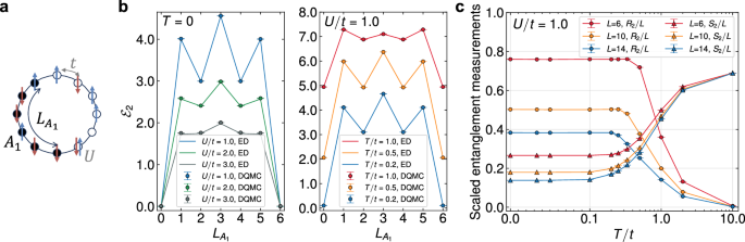
a A schematic illustration of the half-filled Hubbard chain with periodic boundary conditions and its bipartition geometry. b The variation of the rank-two RN \({{{{\mathcal{E}}}}}_{2}\) for a six-site Hubbard chain is depicted as a function of the subsystem length \({L}_{{A}_{1}}\). The solid lines represent the ED results, which agree with the DQMC results at both zero temperature (left panel) and finite temperatures (right panel). c Quantum-classical crossover. The scaled RNR R2/L and EE S2/L of the half-filled Hubbard chain under a half-chain bipartition (i.e., we take \({L}_{{A}_{1}}=L/2\)) vary as functions of temperature. As the temperature rises, the scaled EE for different lengths increases and converges, indicating a dominance of volume law at high temperatures. Meanwhile, the RNR begins to vanish once the temperature reaches a critical value associated with the finite-size gap 1/L44. The error bars in (b) and (c) represent the standard errors from Monte Carlo sampling.
We define the rank-n RN as
$${{{{\mathcal{E}}}}}_{n}=-\frac{1}{n-1}\ln {\mbox{Tr}}\,\left[{\left({\rho }^{{T}_{2}^{f}}\right)}^{n}\right],$$
(8)
where the n-th moment of the PTDM, denoted as \(\,{\mbox{Tr}}\,[{({\rho }^{{T}_{2}^{f}})}^{n}]\), is also referred to as the replica approach of negativity in previous studies19,20. The quantity \({{{{\mathcal{E}}}}}_{n}\) is formally a direct analog to rank-n Rényi EE \({S}_{n}({A}_{1})=-(\ln {{{\rm{Tr}}}}{\rho }_{{A}_{1}}^{n})/(n-1)\), where \({\rho }_{{A}_{1}}={{{{\rm{Tr}}}}}_{{A}_{2}}\rho\) represents the reduced density operator obtained after tracing out subsystem A2. Utilizing Eq. (5), we can derive the DQMC expression for measuring, for instance, the rank-two RN
$${{{{\mathcal{E}}}}}_{2}=-\ln \left\{{\sum }_{{{{{\bf{s}}}}}_{1}{{{{\bf{s}}}}}_{2}}{P}_{{{{{\bf{s}}}}}_{1}}{P}_{{{{{\bf{s}}}}}_{2}}\det \left[{G}^{{{T}_{2}^{f}}}_{{{{{\bf{s}}}}}_{1}}{G}_{{{{{\bf{s}}}}}_{2}}^{{T}_{2}^{f}}+\left(I-{G}_{{{{{\bf{s}}}}}_{1}}^{{T}_{2}^{f}}\right)\left(I-{G}_{{{{{\bf{s}}}}}_{2}}^{{T}_{2}^{f}}\right)\right]\right\}.$$
(9)
The distinction between the FPT and the conventional one is presented herein. For bosonic systems, considering that \({{{\rm{Tr}}}}[{({\rho }^{{T}_{2}})}^{2}]={{{\rm{Tr}}}}[{\rho }^{2}]\), the rank-two RN becomes trivial, thereby rendering the minimal meaningful rank as three19,20,30. However, we show in the occupation number representation that all fermionic PTDMs satisfy \({{{\rm{Tr}}}}[{({\rho }^{{T}_{2}^{f}})}^{2}]={{{\rm{Tr}}}}[{(\rho {\hat{X}}_{2}(\pi ))}^{2}]\) with \({\hat{X}}_{2}\left(\theta \right)={e}^{{{{\rm{i}}}}\theta {\sum }_{j\in {A}_{2}}{n}_{j}}\) being the disorder operator (see the Supplementary Note 1 for details). Consequently, \({{{{\mathcal{E}}}}}_{2}\) can reveal the entanglement information of the system. As shown in Fig. 2b, the results calculated by DQMC and ED show strong agreement in both the zero-temperature and the finite-temperature regimes. In the former regime, the pattern of the rank-two RN exhibits analogous variations to those of the rank-two Rényi EE46,52, in response to alterations in the length of subsystem A1, denoted as \({L}_{{A}_{1}}\). However, at finite temperatures, the negativity maintains a symmetric pattern, which is different from the behavior of EE52,53. As the temperature rises, the magnitude of the negativity increases, resulting in an overall non-zero shift corresponding to a non-zero thermodynamic entropy of \(-\ln ({{{\rm{Tr}}}}{\rho }^{2})\).
Based on the above observation at finite temperatures, we also examine the ratio between \(\,{\mbox{Tr}}\,[{({\rho }^{{T}_{2}^{f}})}^{n}]\) and Tr[ρn] dubbed the Rényi negativity ratio (RNR)23,28,30
$${R}_{n}=-\frac{1}{n-1}\ln \left\{\frac{\,{\mbox{Tr}}\,\left[{\left({\rho }^{{T}_{2}^{f}}\right)}^{n}\right]}{\,{\mbox{Tr}}\,[{\rho }^{n}]}\right\}={{{{\mathcal{E}}}}}_{n}-{S}_{n}^{{{{\rm{th}}}}},$$
(10)
where \({S}_{n}^{{{{\rm{th}}}}}=-(\ln {{{\rm{Tr}}}}{\rho }^{n})/(n-1)\) denotes the thermodynamic Rényi entropy, which equals \({{{{\mathcal{E}}}}}_{n}\) for either A1 = A or A2 = A. A faithful description of mixed-state entanglement necessitates the exclusion of the thermodynamic Rényi entropy \({S}_{n}^{{{{\rm{th}}}}}\). In Fig. 2c, we display the variations of the RNR and EE with temperature for three distinct lengths, namely L = 6, 10, 14. Here, the subsystem A1 is chosen to be half of the chain, yielding an equal bipartition. As the temperature rises, the EE increases while the RNR asymptotically diminishes to zero for all lengths. This serves as a compelling physical demonstration of the quantity Rn. In a generic mixed state, both quantum and classical correlations are present, and effective measurement of mixed-state entanglement should exclusively isolate the quantum correlations15. In the specific context of finite-temperature Gibbs states, the classical correlation is simply the thermal fluctuations delineated by the thermodynamic entropy \({S}_{n}^{{{{\rm{th}}}}}\). Furthermore, at sufficiently low temperatures, the RNR remains constant and establishes a plateau, the length of which is associated with the finite-size gap 1/L44. As depicted in Fig. 2c, it is evident that with an increase in chain length, the plateau becomes narrower. In summary, the monotonic decay of the RNR with rising temperature signifies a crossover from a quantum entangled state to a classical mixed state.
Finite temperature transition in t-V model
To demonstrate the efficacy of the RNR in detecting finite-temperature phase transition, we further consider the half-filled spinless t-V model on a square lattice with periodic boundary conditions53,54,55,
$$H=-t{\sum }_{\langle i,j\rangle }({c}_{i}^{{{\dagger}} }{c}_{j}+{c}_{j}^{{{\dagger}} }{c}_{i})+V{\sum }_{\langle i,j\rangle }\left({n}_{i}-\frac{1}{2}\right)\left({n}_{j}-\frac{1}{2}\right),$$
(11)
where both the hopping and the interaction involve only nearest neighbors (see Fig. 3a for illustration). In the presence of a finite coupling parameter V, this model exhibits a charge density wave (CDW) ground state and undergoes a phase transition from the CDW phase to a metallic phase at finite temperature (see Fig. 3b), with critical behavior falling within the 2D Ising universality class55,56. In the following, we focus on a specific coupling strength, V/t = 2, where the critical temperature was estimated to be Tc/t ≈ 1.055.
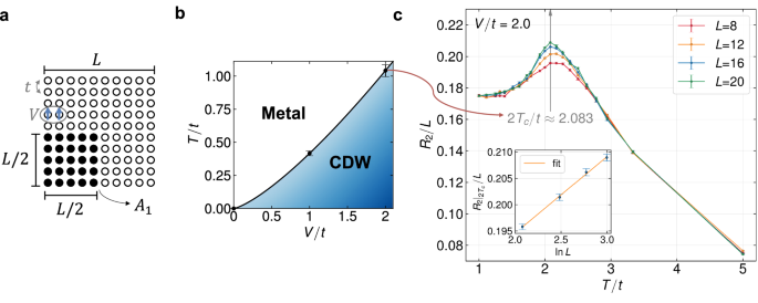
a A schematic illustration of the spinless (or spin-polarized) t-V model on a square lattice and the chosen one-quarter bipartition geometry. b The phase diagram of the t-V model, where the phase boundary points at V = 1 and V = 2 are determined through mixed-state entanglement studies. One can find the data of V = 1 case in the Supplementary Fig. 2. The error bars for these two points are estimated based on the difference between the neighboring temperature points that were calculated. c The finite-temperature transition in the spinless t-V model is detected by the area-law coefficient of the RNR as a function of temperature. A gray vertical arrow indicates the position of the shared peak, with half of its magnitude aligning with the transition point determined in previous studies53,55. The inset shows the linear scaling of the area-law coefficient at the critical point with \(\ln L\). The error bars in (c) represent the standard errors from Monte Carlo sampling.
This model is also a sign-problem-free model57,58,59,60. However, for models with larger dimensions or stronger interaction strengths, the direct sampling of RN using Eq. (9) becomes inaccurate, as a result of the occurrence of spikes61 or the non-Gaussian distribution of Grover determinants \(\det {g}_{x}=\det [{G}_{{{{{\bf{s}}}}}_{2}}^{{T}_{2}^{f}}{G}_{{{{{\bf{s}}}}}_{2}}^{{T}_{2}^{f}}+(I-{G}_{{{{{\bf{s}}}}}_{1}}^{{T}_{2}^{f}})(I-{G}_{{{{{\bf{s}}}}}_{2}}^{{T}_{2}^{f}})]\)62. We implement an incremental algorithm for the RN, analogous to the controllable incremental algorithm for EE62,63,64, the spirit of which is to measure \({(\det {g}_{x})}^{1/{N}_{{{{\rm{inc}}}}}}\) instead of \((\det {g}_{x})\) to circumvent the sampling of an exponentially small quantity with exponentially large variance (see “Methods”). It is important to note that there is a sign ambiguity in the Ninc-th root. In the Supplementary Note 5, we prove that the Grover determinant \(\det {g}_{x}\) is always real and non-negative for two classes of sign-free models, represented by the Hubbard model and the spinless t-V model, respectively.
As illustrated in Fig. 3a, we designate the lower left corner with dimensions (L/2) × (L/2) as subsystem A1, resulting in an area-law coefficient of the RNR of R2/L. The main plot of Fig. 3c presents R2/L as a function of temperature for various system sizes, demonstrating a notably distinct finite-size characteristic compared to the intersection of mutual information53,65. Remarkably, unlike the Hubbard model in Fig. 2c or the previous study on the 2 + 1D transverse field Ising model30, the RNR does not exhibit a monotonic decrease with rising temperature. Instead, for varying lattice sizes, a shared local maximum appears at approximately twice the transition temperature, 2Tc/t ≈ 2.1. The inclusion of the prefactor 2 aligns with the rank of the RNR under consideration, consistent with earlier discussion on the critical behavior within replica approach30,33,35. In general, the singularity of Rn is anticipated to occur at T = nTc with Tc being the physical transition temperature. This expectation arises because Rn, as indicated by the denominator in its definition in Eq. (10), i.e., \({{{\rm{Tr}}}}[{e}^{-n\beta H}]\), effectively corresponds to a Gibbs state with an effective inverse temperature of nβ. Therefore, we demonstrate that it is possible to quantitatively extract the finite-temperature transition points and the phase diagram of the t-V model (see Fig. 3B) from mixed-state entanglement studies. Finally, we briefly highlight the finite-size scaling of the rank-two RNR. As shown in the inset of Fig. 3c, the peaks of R2/L exhibit a logarithmic divergence with system size L, while the area law is well-preserved in regions far from the critical point. This beyond-area-law scaling around the finite temperature critical point is also observed for other values of V (namely, V = 0 and V = 1), a different bipartite geometry, and a different lattice. Refer to the Supplementary Fig. 2 for additional complementary plots.