Single crystals of Cs8RbK3Ti12F48 were grown using alkali metal chlorides as flux. For starting materials, alkali metal fluorides and chlorides were dried, and TiF3 was purified before use. All the materials were mixed and loaded into a Ni crucible, which was then heated to 800 °C and slowly cooled at a rate of 2 °C/h under an Ar atmosphere. The flux was then removed using water to isolate the single crystals. The typical size of the resulting single crystals was ≈ 4 × 4 × 1 mm3 as shown in Supplementary Fig. 1. Three largest single crystals with a total mass of ~1 g were co-mounted for neutron scattering measurements.
Structural analysis of the single crystal was performed using a DIP3200 x-ray diffractometer (XRD) (Bruker AXS) with a Mo target. The structural parameters, including anisotropic displacement parameters, were refined using the full matrix least-square method as implemented in SHELXL-97. The observed and calculated nuclear structure factors, \(\left|{F}_{{obs}}\right|\) and \(\left|{F}_{{calc}}\right|\), respectively, are plotted against each other in Fig. 8. According to the refinement, Cs8RbK3Ti12F48 has a space group of R3m that lacks inversion symmetry. In Supplementary Tables 1 and 2, all structural parameters such as the unit cell constants, the atomic coordinates, and the room temperature isotropic displacement parameters are provided using hexagonal notation. Supplementary Fig. 2a shows a polyhedral representation of the crystal structure where the Ti-F octahedra layers are separated from each other by Rb-Cs-F layers. Supplementary Fig. 2b highlights the kagome lattice formed by the Ti-F octahedra. In hexagonal notation, the kagome planes are the crystallographic ab plane.
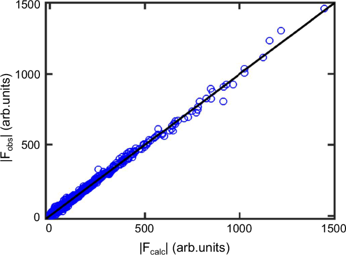
The observed and calculated nuclear structure factors, \(\left|{F}_{{obs}}\right|\) and \(\left|{F}_{{calc}}\right|\), respectively, are plotted against each other.
Density functional theory and magnetic exchange couplings
Based on the crystal structure determined by the x-ray refinement that is summarized in Supplementary Tables 1 and 2, we performed density functional theory (DFT) calculations with OPENMX to estimate the exchange coupling strengths, J, for the four distinct near neighbor Ti3+ pairs. The parametrization of Perdew and Zunger for the local density approximation (LDA) was chosen for the exchange-correlation functional42. The on-site Coulomb interactions were treated via a simplified DFT + U formalism. The hoping parameter t was obtained using the maximally localized Wannier orbital formalism43.
The exchange coupling constants J for Cs2BTi3F12 (B = K, Na, Li) and Rb2NaTi3F12 were calculated using a mapping method that requires quantum calculation of a supercell as reported in refs. 20,21. Since Cs8RbK3Ti12F48 has a chemical unit cell that is 2 × 2 larger than for those four systems, the mapping method is difficult to apply. Instead, we evaluated the exchange constant assuming that the coupling strength is mainly governed by the transfer integral t for each bond. Firstly, we calculated the values of t for Cs2BTi3F12 (B = K, Na, Li) and Rb2NaTi3F12, and plotted their reported J values obtained by the mapping method as a function of \({t}^{2}\). As shown in Supplementary Fig. 3a, the J values show a good linear relation with \({t}^{2}\): \(\frac{J}{K}=6.64\,{\left(\frac{t}{{\mathrm{meV}}}\right)}^{2}-40.26\). We then calculated t for the near neighbor Ti3+-Ti3+ spin pairs in Cs8RbK3Ti12F48, and obtained estimates for J from this formula. Supplementary Fig. 3b shows the modulated kagome lattice of Cs8RbK3Ti12F48 with the estimated J. The red solid, red dashed, blue solid, and blue dashed lines represent the exchange interaction strengths of J = (7.4, 6.3, 5.1, 3.9) meV, respectively. Note that there are triangles with uniform Js (represented by blue solid lines or by red dashed lines) and triangles with nonuniform Js (represented by two different types of lines). We would like to stress here that this simple DFT estimation of Js should be used only as a starting point for further detailed DFT studies of this compound.
Bulk magnetization and specific heat measurements
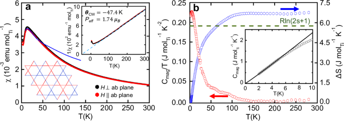
Bulk magnetization and specific heat measurements were performed on a single crystal using a Quantum Design MPMS-XL system and a PPMS-14LHS system (Quantum Design), respectively, at the Research Center for Low Temperature and Materials Science, Kyoto University. Magnetic susceptibility measurement for the zero-field cooled (ZFC) condition was conducted in a heating process at the rate of 1.5 K/min below 60 K and at the rate of 3 K/min above 60 K. The field cooled (FC) data was taken in a cooling process at the same rates as those used for the ZFC data (Fig. 9). The Curie-Weiss temperature was determined by fitting the bulk susceptibility data between 100 K and 300 K. The rise of \(\chi (T)\) below 3.5 K is due to unavoidable imperfections in real crystals. The inferred molar abundance is approximately 1%. Heat capacity was measured at each temperature using a relaxation method with temperature rise of 2%. After that, the sample was heated to the next measuring temperature at the rate of 0.5-5 K/min, and the measurement was commenced when temperature became stable.
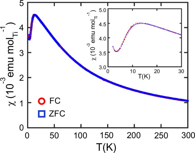
χ was measured under magnetic field of 1 Tesla. In the FC process, the sample was cooled under 1 Tesla. The inset shows the data up to 30 K. The data show no FC-ZFC hysteresis.
Neutron scattering measurements
The Time-Of-Flight (TOF) neutron scattering experiment was conducted using the 4D-Space Access Neutron Spectrometer (4SEASONS) at the Japan Proton Accelerator Research Complex (J-PARC) Materials and Life Science Experimental Facility, Tokai, Japan44. The experiment was carried out on three single crystals that were co-aligned and attached using CYTOP (CTL-107M) to Al plates that in turn were attached to an Al sample holder. The total sample mass was \(\sim 1\,g\). The Al sample holder was mounted in a 4He cryostat with a 1.5 K base temperature. The crystals were mounted with the crystallographic c axis parallel with the incident neutron beam, which allowed us to integrate the intensity along the c axis perpendicular to the kagome plane. At 4SEASONS, the neutron scattering data were collected simultaneously using five different incident neutron energies of \({E}_{i}=\) (3, 4, 6, 10, 19) meV45. These incident energies provided full width at half maximum energy resolutions of (0.11, 0.17, 0.27, 0.51, 1.20) meV, respectively, at the elastic line. This allowed us to map inelastic scattering over the entire band of magnetic excitations up to 15 meV with appropriate energy resolution throughout. Data were acquired at two temperatures, 1.5 K and 20 K, to examine spin fluctuations below and above the cross-over temperature T*. At the end of the experiment, the empty cryostat without the crystals was measured for background subtraction using the same experimental setup. The data were analyzed using the Utsusemi software package46.
Absolute normalization of magnetic neutron scattering data
Normalization of the neutron scattering intensity data to absolute units for the scattering cross section can be accomplished through comparison to well-known standards including incoherent elastic scattering from vanadium, sample incoherent elastic scattering, sample elastic nuclear peaks, and sample phonon scattering47. We used the sample incoherent elastic scattering as described in Supplementary Information.
Symmetrization of neutron scattering data
In neutron scattering experiment, we could measure S(Q) over a limited area in the momentum space as shown in Supplementary Fig. 5a as an example. Utilizing that magnetic scattering in Cs8RbK3Ti12F48 has a six-fold symmetry, we constructed S(Q) over the 360o angular range as shown in Supplementary Fig. 5b, which provides a comprehensive representation of S(Q) across the entire angular range.
Damped linear spin wave theory
Linear spin wave (LSW) analysis is done on a long-range ordered q = 0, \( 120^{{\circ }}\) state with the minimal spin Hamiltonian:
$${{{\mathscr{H}}}}=J\sum\limits_{ }{s}_{i}\cdot {s}_{j}+\sum\limits_{ }{{{{\boldsymbol{D}}}}}_{{ij}}\cdot \left({s}_{i}\times {s}_{j}\right)$$
where \(J=8.7\) meV and \({{{{\boldsymbol{D}}}}}_{{ij}}=D\hat{z}\) with D = 0.23 meV. A q = 0, 120° state can be represented by a three-sublattice state within each unit cell:
$${s}_{i,A}=\left(-\frac{\sqrt 3}{2},-\frac{1}{2},0\right),\,{s}_{i,B}=\left(\frac{\sqrt 3}{2},-\frac{1}{2},0\right),{s}_{i,C}=\left(0,1,0\right).$$
Transformation to the spin fully polarized local coordinates \({s}_{i,A}={R}_{A}{\widetilde{s}}_{i,A}\), \({s}_{i,B}={R}_{B}{\widetilde{s}}_{i,B}\), \({s}_{i,C}={R}_{C}{\widetilde{s}}_{i,C}\) is accomplished with the following rotation matrices:
$${R}_{A}=\left(\begin{array}{ccc}\frac{1}{4} & -\frac{\sqrt{3}}{4} & \frac{\sqrt{3}}{2}\\ -\frac{\sqrt{3}}{4} & \frac{3}{4} & -\frac{1}{2}\\ \frac{\sqrt{3}}{2} & \frac{1}{2} & 0\end{array}\right),{R}_{B}=\left(\begin{array}{ccc}\frac{1}{4} & \frac{\sqrt{3}}{4} & \frac{\sqrt{3}}{2}\\ \frac{\sqrt{3}}{4} & \frac{3}{4} & -\frac{1}{2}\\ -\frac{\sqrt{3}}{2} & \frac{1}{2} & 0\end{array}\right),{R}_{C}=\left(\begin{array}{ccc}1 & 0 & 0\\ 0 & 0 & 1\\ 0 & -1 & 0\end{array}\right).$$
The Holstein-Primakoff (HP) transformation48 rewrites spin operators in the fully polarized local coordinates in terms of HP bosons where we can expand \({\widetilde{s}}_{i}^{x}\) and \({\widetilde{s}}_{i}^{y}\) to linear order of 1/s:
$${\widetilde{s}}_{i,\alpha }^{x}\approx \sqrt{\frac{s}{2}}({a}_{i,\alpha }+{a}_{i,\alpha }^{{{\dagger}} }),{\widetilde{s}}_{i,\alpha }^{y}\approx -i\sqrt{\frac{s}{2}}({a}_{i,\alpha }-{a}_{i,\alpha }^{{{\dagger}} }),{\widetilde{s}}_{i,\alpha }^{z}=s-{a}_{i,\alpha }^{{{\dagger}} }{a}_{i,\alpha }.$$
After transforming the HF bosons in the momentum space, we obtain:
$${{{{\mathscr{H}}}}}_{{LSW}}={Js}\sum\limits_{{{{\boldsymbol{k}}}}}{A}_{{{{\boldsymbol{k}}}}}^{{{\dagger}} }{M}_{{{{\boldsymbol{k}}}}}{A}_{{{{\boldsymbol{k}}}}},$$
where \({A}_{{{{\boldsymbol{k}}}}}^{{{\dagger}} }=\left({a}_{{{{\boldsymbol{k}}}},A}^{{{\dagger}} },{a}_{{{{\boldsymbol{k}}}},B}^{{{\dagger}} },{a}_{{{{\boldsymbol{k}}}},C}^{{{\dagger}} },{a}_{-{{{\boldsymbol{k}}}},A},{a}_{-{{{\boldsymbol{k}}}},B},{a}_{-{{{\boldsymbol{k}}}},C}\right)\) and
$${M}_{{{{\boldsymbol{k}}}}}=\left(\begin{array}{cc}{B}_{{{{\boldsymbol{k}}}}} & {C}_{{{{\boldsymbol{k}}}}}^{{{\dagger}} }\\ {C}_{{{{\boldsymbol{k}}}}} & {B}_{-{{{\boldsymbol{k}}}}}^{T}\end{array}\right)$$
with
$${B}_{{{{\boldsymbol{k}}}}}=\left(\begin{array}{ccc}1+\sqrt{3}\frac{D}{J} & -\frac{{e}^{i\frac{\pi }{3}}\left(1+{e}^{-i{{{{\boldsymbol{v}}}}}_{1}\cdot {{{\boldsymbol{k}}}}}\right)}{8}\left(1-\sqrt{3}\frac{D}{J}\right) & \frac{{e}^{i\frac{2\pi }{3}}\left(1+{e}^{-i{{{{\boldsymbol{v}}}}}_{2}\cdot {{{\boldsymbol{k}}}}}\right)}{8}\left(1-\sqrt{3}\frac{D}{J}\right)\\ -\frac{{e}^{-i\frac{\pi }{3}}\left(1+{e}^{-i{{{{\boldsymbol{v}}}}}_{1}{{\cdot }}{{{\boldsymbol{k}}}}}\right)}{8}\left(1-\sqrt{3}\frac{D}{J}\right) & 1+\sqrt{3}\frac{D}{J} & -\frac{{e}^{i\frac{\pi }{3}}\left(1+{e}^{-i{{{{\boldsymbol{v}}}}}_{3}\cdot {{{\boldsymbol{k}}}}}\right)}{8}\left(1-\sqrt{3}\frac{D}{J}\right)\\ \frac{{e}^{-i\frac{2\pi }{3}}\left(1+{e}^{-i{{{{\boldsymbol{v}}}}}_{2}\cdot {{{\boldsymbol{k}}}}}\right)}{8}\left(1-\sqrt{3}\frac{D}{J}\right) & -\frac{{e}^{-i\frac{\pi }{3}}\left(1+{e}^{i{{{{\boldsymbol{v}}}}}_{3}\cdot {{{\boldsymbol{k}}}}}\right)}{8}\left(1-\sqrt{3}\frac{D}{J}\right) & 1+\sqrt{3}\frac{D}{J}\end{array}\right),$$
$${C}_{{{{\boldsymbol{k}}}}}=\frac{\sqrt{3}}{8}\left(\sqrt{3}+\frac{D}{J}\right)\left(\begin{array}{ccc}0 & -\left(1+{e}^{-i{{{{\boldsymbol{v}}}}}_{1}\cdot {{{\boldsymbol{k}}}}}\right) & {e}^{i\frac{\pi }{3}}\left(1+{e}^{-i{{{{\boldsymbol{v}}}}}_{2}\cdot {{{\boldsymbol{k}}}}}\right)\\ -\left(1+{e}^{i{{{{\boldsymbol{v}}}}}_{1}\cdot {{{\boldsymbol{k}}}}}\right) & 0 & {e}^{-i\frac{\pi }{3}}\left(1+{e}^{-i{{{{\boldsymbol{v}}}}}_{3}\cdot {{{\boldsymbol{k}}}}}\right)\\ {e}^{i\frac{\pi }{3}}\left(1+{e}^{i{{{{\boldsymbol{v}}}}}_{2}\cdot {{{\boldsymbol{k}}}}}\right) & {e}^{-i\frac{\pi }{3}}\left(1+{e}^{i{{{{\boldsymbol{v}}}}}_{3}\cdot {{{\boldsymbol{k}}}}}\right) & 0\end{array}\right)$$
and \({{{{\boldsymbol{v}}}}}_{1}=\left(2,0,0\right)\), \({{{{\boldsymbol{v}}}}}_{2}=(1,\sqrt{3},0)\), \({{{{\boldsymbol{v}}}}}_{3}=(-1,\sqrt{3},0)\).
Using Bogoliubov transformation for bosons49 to diagonalize the Hamiltonian at \({{{\boldsymbol{k}}}}=0\), we obtain the energy of the dispersionless mode:
$$\varDelta={Js}\left(3\sqrt{2}\sqrt{\frac{D}{J}\left(\frac{D}{J}+\frac{1}{\sqrt{3}}\right)}\right)\approx 2.67\;{{{\rm{meV}}}},$$
and similarly, diagonalizations at \({{{\boldsymbol{k}}}}={\left({{\mathrm{1,0}}}\right)}_{{{{\rm{Ti}}}}}\) and \({\left(\frac{4}{3},\frac{4}{3}\right)}_{{{{\rm{Ti}}}}}\) yield the maximum of two dispersive modes:
$${{{\hslash }}\omega }_{{{{\boldsymbol{M}}}},{{{\rm{top}}}}}=2{Js}\left(1+\sqrt{3}\frac{D}{J}\right)\approx 9.1{{{{\rm{meV}}}}},$$
$${{{\hslash }}\omega }_{{{{\boldsymbol{K}}}},{{{\rm{top}}}}}={Js}\sqrt{\frac{3}{2}}\sqrt{3+6\frac{{D}^{2}}{{J}^{2}}+5\sqrt{3}\frac{D}{J}}\approx 9.6{{{{\rm{meV}}}}}$$
along the \((H,0)\) and \((H,H)\) directions, respectively.
Next, we use the results from LSW analysis to compute the neutron scattering intensity. The magnetic neutron scattering intensity is computed by50:
$$S({{{\boldsymbol{Q}}}},\omega )\propto {F({{{\boldsymbol{Q}}}})}^{2}\sum\limits_{\mu \nu }\left({\delta }_{\mu \nu }-\frac{{Q}_{\mu }{Q}_{\nu }}{{\left|{{{\boldsymbol{Q}}}}\right|}^{2}}\right){s}^{\mu \nu }\left({{{\boldsymbol{Q}}}},\omega \right),$$
where \(F({{{\bf{Q}}}})\) denotes the form factor for Ti3+, \({Q}_{\mu },{Q}_{\nu }\) are the μ,ν components of the Q vector, and most importantly, \({s}^{\mu \nu }\left({{{\bf{Q}}}},\omega \right)\) is the dynamical structure factor:
$${s}^{\mu \nu }\left({{{\bf{Q}}}},\omega \right)=\sum\limits_{\alpha \beta }\int {dt}\;{e}^{-i\omega t}\left\langle {s}_{\alpha }^{\mu }{\left(-{{{\bf{Q}}}},0\right)s}_{\beta }^{\nu }\left({{{\bf{Q}}}},t\right)\right\rangle,$$
which can be computed in terms of Bogoliubov bosonic quasiparticle correlations obtained from LSW analysis:
$$\left\langle {b}_{\alpha,{{{\boldsymbol{k}}}}}^{{{\dagger}} }\left(t\right){b}_{\beta,{{{{\boldsymbol{k}}}}}^{{\prime} }}\left(0\right)\right\rangle={\delta }_{\alpha \beta }{\delta }_{{{{\boldsymbol{k}}}}{{{{\boldsymbol{k}}}}}^{{\prime} }}n\left({\omega }_{\alpha,{{{\boldsymbol{k}}}}}\right){e}^{-i{\omega }_{\alpha,{{{\boldsymbol{k}}}}}t},$$
$$\left\langle {b}_{\alpha,{{{\boldsymbol{k}}}}}(0){b}_{\beta,{{{\boldsymbol{k}}}}{\prime} }^{{{\dagger}} }\left(t\right)\right\rangle={\delta }_{\alpha \beta }{\delta }_{{{{\boldsymbol{kk}}}}{\prime} }\left[n({\omega }_{\alpha,{{{\boldsymbol{k}}}}})+1\right]{e}^{i{\omega }_{\alpha,{{{\boldsymbol{k}}}}}t},$$
with the Bose factor \(n\left({\omega }_{\alpha,{{{\boldsymbol{k}}}}}\right)={\left[{e}^{\hslash {\omega }_{\alpha,{{{\boldsymbol{k}}}}}/({k}_{B}T)}-1\right]}^{-1}\), where the momentum k is within the magnetic Brillouin zone such that Q-k gives integer multiples of the reciprocal lattice vectors. At T = 0, we have \(n\left({\omega }_{\alpha,{{{\boldsymbol{k}}}}}\right)=0\), so only the second term contributes to the dynamical structure factor. For generic k points, the LSW Hamiltonian is diagonalized numerically, so the transformations between spin operators and Bogoliubov quasiparticles are also obtained at each k point numerically.
To account for the finite lifetime of the single magnon excitation, we introduce a broadening factor (or energy uncertainty) proportional to the energy of the magnon mode \({\delta \epsilon }_{\alpha,{{{\boldsymbol{k}}}}}\propto {\epsilon }_{\alpha,{{{\boldsymbol{k}}}}}\) for a finite magnon lifetime \({\tau }_{\alpha,{{{\boldsymbol{k}}}}}=\frac{\hslash }{2{\delta \epsilon }_{\alpha,{{{\boldsymbol{k}}}}}}\) such that \({\epsilon }_{\alpha,{{{\boldsymbol{k}}}}}\) is replaced by \({\epsilon }_{\alpha,{{{\boldsymbol{k}}}}}+i{\delta \epsilon }_{\alpha,{{{\boldsymbol{k}}}}}\). This gives rise to the following form of the dynamic correlation function:
$$S({{{\bf{Q}}}},\omega )=\frac{{F({{{\bf{Q}}}})}^{2}}{\pi }\sum\limits_{\mu \nu,\alpha }\left({\delta }_{\mu \nu }-\frac{{Q}_{\mu }{Q}_{\nu }}{{\left|{{{\bf{Q}}}}\right|}^{2}}\right){\left[{L}_{{{{\boldsymbol{k}}}}}^{\mu \nu }\right]}_{\alpha+3,\alpha+3}\frac{{\delta \epsilon }_{\alpha,{{{\boldsymbol{k}}}}}}{{{\delta \epsilon }_{\alpha,{{{\boldsymbol{k}}}}}}^{2}+{\left({{\hslash }}\omega -{\epsilon }_{\alpha,{{{\boldsymbol{k}}}}}\right)}^{2}},$$
where \({L}_{{{{\boldsymbol{k}}}}}^{\mu \nu }\) denotes the numerical transformation between the spin operators and the Bogoliubov bosonic quasiparticle operators (the subscript α + 3 indicates the summation is only over the lower half diagonal elements at T = 0).
Calculation for the finite-temperature neutron response
The finite-temperature neutron scattering intensity \(S({{{\bf{Q}}}},\omega )\) can be computed through simulating the system using Landau-Lifshitz dynamics (LLD):
$$\frac{d{s}_{i}}{{dt}}={-s}_{i}{{{\rm{\times }}}}{B}_{i}$$
where the effective field is \({B}_{i}=-d{{{\mathscr{H}}}}{{/}}d{s}_{i}\) and \({{{\mathscr{H}}}}\) is the spin Hamiltonian. For a given initial state \(\{{s}_{i}\left(t=0\right)\}\), the above LL equation can be integrated to produce “trajectories” of spins \(\left\{{s}_{i}\left(t\right)\right\}.\) The information of excited states in the initial state is encoded in these trajectories. To this end, we write the lattice site index as \(i=({{{\boldsymbol{R}}}},\alpha )\), where R is the position vector of a given unit cell and α is the sublattice index. The Fourier transform of the spin trajectories are given by:
$${s}_{\alpha }\left({{{\boldsymbol{Q}}}},t\right)=\frac{1}{\sqrt{N}}\sum\limits_{i}{s}_{\alpha }\left({{{\boldsymbol{R}}}},t\right){e}^{-i{{{\boldsymbol{Q}}}}\cdot {{{\boldsymbol{R}}}}},$$
The dynamical structure factor is then given by:
$${s}^{\mu \nu }\left({{{\bf{Q}}}},\omega \right)=\sum\limits_{\alpha \beta }\int {dt}\;{e}^{-i\omega t}\left\langle {s}_{\alpha }^{\mu }{\left(-{{{\bf{Q}}}},0\right)s}_{\beta }^{\nu }\left({{{\bf{Q}}}},t\right)\right\rangle,$$
Importantly, here the expectation value \(\left\langle \cdots \right\rangle\) is taken over the different initial conditions which are sampled either using Monte Carlo simulations or stochastic Landau-Lifshitz-Gilbert simulations at a given temperature T. It is worth noting that the system energy is conserved in LLD. The dependence on temperature, which in turn determines the degree of spin fluctuations, solely comes from the sampled initial states. Moreover, since the sampled initial spins could be in a classical liquid phase, the LLD approach does not require the assumption of a long-range magnetic order. As a result, LLD methods have been employed in the calculation of \({s}^{\mu \nu }\left({{{\bf{Q}}}},\omega \right)\) for classical spin liquids such as in frustrated magnets. Using the LLD methods provided in the SUNNY package (https://github.com/SunnySuite/Sunny.jl), we computed the intensity of magnetic inelastic neutron scattering \(S({{{\bf{Q}}}},\omega )\) from 15 independent simulation runs with \(N=100{\times }100{\times }3\) spins at T = 1.5 K, 2.2 K, and 3.0 K.
Dimer and trimer models
In neutron scattering work on herbertsmithite, ZnCu3(OH)6Cl25, the energy integrated magnetic response function was successfully compared to a noninteracting dimer model. The associated non-dispersive “local” form of the response function2 might be associated with a disordered random singlet state or spinon-vison interactions36. In our experiments on Cs8RbK3Ti12F48 it has been possible to cover the entire range of the magnetic bandwidth for a kagome material, which may allow distinguishing such scenarios.
Here we examine whether our neutron scattering data for Cs8RbK3Ti12F48 are consistent with local excitations as for a random singlet phase. Two local excitations were considered, dimers and 120° trimers. Firstly, we found that the models of dimers and trimers yield the same magnetic structure factor, i.e., they are not distinguishable through neutron scattering. Secondly, the energy integrated equal time magnetic response function measured for Cs8RbK3Ti12F48 cannot be reproduced by the local dimer/trimer model. Though damped linear spin wave theory cannot account for the broad continuum scattering, it describes the equal-time response function better than local models of dimers and trimers.
As shown in Supplementary Fig. 6a, considering their phase factors there are two types of 120° trimers where three spins form a 120° spin configuration as shown in the inset. The magnetic structure factor of the first trimer circled by the red dashed line is:
$${{{{\boldsymbol{F}}}}}_{{trimer},1}\left(h,k\right)=\left|{{{\boldsymbol{A}}}}\right|{e}^{i\pi k}\hat{y}+\left|{{{\boldsymbol{B}}}}\right|{e}^{i\frac{\pi }{2}\left(h+2k\right)}\left(-\frac{\sqrt{3}}{2}\hat{x}-\frac{1}{2}\hat{y}\right)+\left|{{{\boldsymbol{C}}}}\right|{e}^{i\frac{\pi }{2}k}\left(\frac{\sqrt{3}}{2}\hat{x}-\frac{1}{2}\hat{y}\right).$$
Or assuming that \(\left|{{{\boldsymbol{A}}}}\right|=\left|{{{\boldsymbol{B}}}}\right|=\left|{{{\boldsymbol{C}}}}\right|=1\),
$${{{{\boldsymbol{F}}}}}_{{trimer},1}\left(h,k\right)={e}^{i\pi k}\left[\left(-\frac{\sqrt{3}}{2}{e}^{i\frac{\pi }{2}h}+\frac{\sqrt{3}}{2}{e}^{-i\frac{\pi }{2}k}\right)\hat{x}+\left(1-\frac{1}{2}{e}^{i\frac{\pi }{2}h}-\frac{1}{2}{e}^{-i\frac{\pi }{2}k}\right)\hat{y}\right].$$
Similarly, for the second trimer circled by the blue dashed line,
$${{{{\boldsymbol{F}}}}}_{{trimer},2}\left(h,k\right)={e}^{i\pi h}\left[\left(-\frac{\sqrt{3}}{2}{e}^{-i\frac{\pi }{2}h}+\frac{\sqrt{3}}{2}{e}^{i\frac{\pi }{2}k}\right)\hat{x}+\left(1-\frac{1}{2}{e}^{-i\frac{\pi }{2}h}-\frac{1}{2}{e}^{i\frac{\pi }{2}k}\right)\hat{y}\right].$$
Thus, the neutron scattering intensity from the two noninteracting trimers becomes:
$${I}_{{trimer}}\left(h,k\right) \propto {\left|{{{{\boldsymbol{F}}}}}_{{trimer},1}\left(h,k\right)\right|}^{2}+{\left|{{{{\boldsymbol{F}}}}}_{{trimer},2}\left(h,k\right)\right|}^{2}\\ \propto \left(3-\cos \frac{\pi }{2}h-\cos \frac{\pi }{2}k-\cos \frac{\pi }{2}(h+k)\right).$$
Supplementary Fig. 6b, on the other hand, shows three types of decoupled dimers. Since the structure factor squared of a dimer is \({\left|{{{{\boldsymbol{F}}}}}_{{dimer}}\left({{{\boldsymbol{Q}}}}\right)\right|}^{2}\propto \left(1-\cos \left({{{\boldsymbol{Q}}}}.{{{\boldsymbol{r}}}}\right)\right)\) 51,52, the neutron scattering intensity from the three noninteracting dimers becomes:
$${I}_{{dimer}}\left(h,k\right) \propto {\left|{{{{\boldsymbol{F}}}}}_{{dimer},1}\left(h,k\right)\right|}^{2}+{\left|{{{{\boldsymbol{F}}}}}_{{dimer},2}\left(h,k\right)\right|}^{2}+{\left|{{{{\boldsymbol{F}}}}}_{{dimer},3}\left(h,k\right)\right|}^{2} \\ \propto \left(1-\cos \frac{\pi }{2}(h+k)\right)+\left(1-\cos \frac{\pi }{2}k\right)+\left(1-\cos \frac{\pi }{2}{h}\right) \\ =\left(3-\cos \frac{\pi }{2}h-\cos \frac{\pi }{2}k-\cos \frac{\pi }{2}(h+k)\right).$$
Therefore, \({I}_{{trimer}}\left(h,k\right)\) and \({I}_{{dimer}}\left(h,k\right)\) are exactly the same and cannot be distinguished by the energy integrated magnetic response function.
Q-dependence of the equal-time response function and propagating excitation
Figure 6a shows a contour map of the experimental equal-time response function \(S\left({{{\bf{Q}}}}\right)={\int }_{0.3{meV}}^{13{meV}}S\left({{{\bf{Q}}}},\hslash \omega \right)d(\hslash \omega )\) at 1.5 K that provides us with important information on the putative quantum spin liquid state of Cs8RbK3Ti12F48. \(S\left({{{\bf{Q}}}}\right)\) exhibits three salient features: A global maximum at \({\Gamma }_{2}\), a strong signal along the \({\Gamma }_{2}\to {M}_{2}\to {\Gamma }_{2}^{\prime}\) direction, and a broad bump near \({K}_{2}\). Figure 6b–f shows \(S\left({{{\bf{Q}}}}\right)\) obtained with different theoretical models as described in the caption. \({S\left({{{\boldsymbol{Q}}}}\right)}_{{dimer}/{trimer}}\) displays a three-fold symmetric peak centered at \({K}_{2}\) and a weaker signal at around \({\Gamma }_{2}\), which is inconsistent with the experimental \(S\left({{{\boldsymbol{Q}}}}\right)\). Consistent with the data, \({S\left({{{\bf{Q}}}}\right)}_{{LSW}}\) for the damped spin-wave model and \({S\left({{{\bf{Q}}}}\right)}_{{LLD}}\) for Landau-Lifshitz dynamics at 1.5 K and 2.2 K, on the other hand, show a strong signal at \({\Gamma }_{2}\). In comparison, \({S\left({{{\bf{Q}}}}\right)}_{{LLD}}\) at 3 K shows similar Q-dependence as \({S\left({{{\boldsymbol{Q}}}}\right)}_{{dimer}/{trimer}}\) does.
For a more detailed comparison of these models with the experimental data, Fig. 7 shows \(S\left({{{\bf{Q}}}}\right)\), \({S\left({{{\bf{Q}}}}\right)}_{{LSW}}\), and \({S\left({{{\bf{Q}}}}\right)}_{{dimer}/{trimer}}\) along the \({{{{{\rm{M}}}}}_{2}\to {\Gamma }_{1}\to \Gamma }_{2}\to {{{{\rm{M}}}}}_{2}\to {{{{\rm{K}}}}}_{2}\) path in the 2D Brillouin zone. \(S\left({{{\bf{Q}}}}\right)\) is strong at \({\Gamma }_{2}\) and along \({\Gamma }_{2}\to {{{{\rm{M}}}}}_{2}\). It is stronger at \({{{{\rm{K}}}}}_{2}\) than at \({{{{\rm{K}}}}}_{1}\). \({S\left({{{\bf{Q}}}}\right)}_{{LSW}}\) and \({S\left({{{\bf{Q}}}}\right)}_{{LLD}}\) at 2.2 K show strong maxima at \({\Gamma }_{2}\) points, while it is sharper than \(S\left({{{\boldsymbol{Q}}}}\right)\) along all directions except \({{{{\rm{M}}}}}_{2}\to {{{{\rm{K}}}}}_{2}\). For \({{{{\rm{M}}}}}_{2}\to {{{{\rm{K}}}}}_{2}\), \(S\left({{{\bf{Q}}}}\right)\) is stronger at \({{{{\rm{M}}}}}_{2}\) than at \({{{{\rm{K}}}}}_{2}\), while \({S\left({{{\bf{Q}}}}\right)}_{{LSW}}\) and \({S\left({{{\bf{Q}}}}\right)}_{{LLD}}\) at 2.2 K are stronger at \({{{{\rm{K}}}}}_{2}\) than at \({{{{\rm{M}}}}}_{2}\). \({S\left({{{\bf{Q}}}}\right)}_{{dimer}/{trimer}}\) reproduces the broad features along \({{{{{\rm{M}}}}}_{2}\to {\Gamma }_{1}\to \Gamma }_{2}\). However, \({S\left({{{\bf{Q}}}}\right)}_{{dimer}/{trimer}}\) does not reproduce the sharp peak of \(S\left({{{\bf{Q}}}}\right)\) centered at \({\Gamma }_{2}\), and contrary to the experimental data for \(\left({{{\boldsymbol{Q}}}}\right)\) yields no modulation along \({\Gamma }_{2}\to {{{{\rm{M}}}}}_{2}\) beyond the \({{{{\rm{Ti}}}}}^{3+}\) form factor. Thus, we conclude that magnetic excitations in Cs8RbK3Ti12F48 are not associated with decoupled dimers or trimers.