The formulation of the problem is as follows:
$$\min \,\,\,\,\,\,F_{1} = \sum\limits_{{\omega \in \Gamma_{S} }} {\sigma_{\omega } \sum\limits_{{\tau \in \Gamma_{OH} }} {\left\{ {\xi_{\tau ,\omega }^{E} P_{o,\tau ,\omega }^{S} + \xi_{\tau ,\omega }^{H} H_{o,\tau ,\omega }^{S} } \right\}} }$$
(1)
Subject to:
$$P_{b,\tau ,\omega }^{S} + \sum\limits_{{h \in \Gamma_{H} }} {A_{b,h}^{E} P_{h,\tau ,\omega }^{H} } – \sum\limits_{{l \in \Gamma_{B} }} {B_{b,l}^{E} P_{b,l,\tau ,\omega }^{L} = P_{b,\tau ,\omega }^{C} } \,\,\,\forall b,\tau ,\omega$$
(2)
$$Q_{b,\tau ,\omega }^{S} – \sum\limits_{{l \in \Gamma_{B} }} {B_{b,l}^{E} Q_{b,l,\tau ,\omega }^{L} = Q_{b,\tau ,\omega }^{C} } \,\,\,\forall b,\tau ,\omega$$
(3)
$$P_{b,l,\tau ,\omega }^{L} = g_{b,l}^{L} \left( {V_{b,\tau ,\omega } } \right)^{2} – V_{b,\tau ,\omega } V_{l,\tau ,\omega } \left\{ {g_{b,l}^{L} \cos \left( {\phi_{b,\tau ,\omega } – \phi_{l,\tau ,\omega } } \right) + b_{b,l}^{L} \sin \left( {\phi_{b,\tau ,\omega } – \phi_{l,\tau ,\omega } } \right)} \right\}\,\,\,\,\forall b,l,\tau ,\omega$$
(4)
$$Q_{b,l,\tau ,\omega }^{L} = – b_{b,l}^{L} \left( {V_{b,\tau ,\omega } } \right)^{2} + V_{b,\tau ,\omega } V_{l,\tau ,\omega } \left\{ {b_{b,l}^{L} \cos \left( {\phi_{b,\tau ,\omega } – \phi_{l,\tau ,\omega } } \right) – g_{b,l}^{L} \sin \left( {\phi_{b,\tau ,\omega } – \phi_{l,\tau ,\omega } } \right)} \right\}\,\,\,\,\forall b,l,\tau ,\omega$$
(5)
$$H_{m,\tau ,\omega }^{S} + \sum\limits_{{h \in \Gamma_{H} }} {A_{m,h}^{H} H_{h,\tau ,\omega }^{H} } – \sum\limits_{{l \in \Gamma_{T} }} {B_{n,l}^{H} H_{m,l,\tau ,\omega }^{L} = H_{m,\tau ,\omega }^{C} } \,\,\,\,\,\,\forall m,\tau ,\omega$$
(6)
$$H_{m,l,\tau ,\omega }^{L} = \varpi_{m,l} \left( {T_{m,\tau ,\omega } – T_{l,\tau ,\omega } } \right)\,\,\,\,\,\,\,\,\,\,\,\,\,\forall m,l,\tau ,\omega$$
(7)
$$\underline{V} \le V_{b,\tau ,\omega } \le \overline{V}\,\,\,\,\,\,\,\,\,\,\,\,\,\forall b,\tau ,\omega$$
(8)
$$\left( {P_{b,l,\tau ,\omega }^{L} } \right)^{2} + \left( {Q_{b,l,\tau ,\omega }^{L} } \right)^{2} \le \left( {\overline{S}_{b,l}^{L} } \right)^{2} \,\,\,\,\,\,\,\,\,\,\,\,\forall b,l,\tau ,\omega$$
(9)
$$\left( {P_{b,\tau ,\omega }^{S} } \right)^{2} + \left( {Q_{b,\tau ,\omega }^{S} } \right)^{2} \le \left( {\overline{S}_{b}^{S} } \right)^{2} \,\,\,\,\,\,\,\,\,\,\,\,\forall b = o,\tau ,\omega$$
(10)
$$\underline{T} \le T_{m,\tau ,\omega } \le \overline{T}\,\,\,\,\,\,\,\,\,\,\,\,\,\forall m,\tau ,\omega$$
(11)
$$- \overline{H}_{m,l}^{L} \le H_{m,l,\tau ,\omega }^{L} \le \overline{H}_{m,l}^{L} \,\,\,\,\,\,\,\,\,\,\,\,\,\forall m,l,\tau ,\omega$$
(12)
$$- \overline{H}_{m}^{S} \le H_{m,\tau ,\omega }^{S} \le \overline{H}_{m}^{S} \,\,\,\,\,\,\,\,\,\,\,\,\,\forall m = o,\tau ,\omega$$
(13)
$$P^{H} ,H^{H} \in \arg \left\{ {\max \,\,\,\,\,\,F_{2} = \sum\limits_{{\omega \in \Gamma_{S} }} {\sigma_{\omega } \sum\limits_{{\tau \in \Gamma_{OH} }} {\sum\limits_{{h \in \Gamma_{H} }} {\left( {\zeta_{\tau ,\omega }^{E} P_{h,\tau ,\omega }^{H} + \zeta_{\tau ,\omega }^{H} H_{h,\tau ,\omega }^{H} } \right)} } } } \right.$$
(14)
Subject to:
$$P_{h,\tau ,\omega }^{H} = P_{h,\tau ,\omega }^{BU} + P_{h,\tau ,\omega }^{WT} + \left( {P_{h,\tau ,\omega }^{Ge} – P_{h,\tau ,\omega }^{Mo} } \right) + \left( {P_{h,\tau ,\omega }^{FC} – P_{h,\tau ,\omega }^{EL} } \right) – P_{h,\tau ,\omega }^{C} :\vartheta_{h,\tau ,\omega }^{P} \,\,\,\,\,\,\forall h,\tau ,\omega$$
(15)
$$H_{h,\tau ,\omega }^{H} = H_{h,\tau ,\omega }^{BU} + \left( {H_{h,\tau ,\omega }^{DCH} – H_{h,\tau ,\omega }^{CH} } \right) – H_{h,\tau ,\omega }^{C} :\vartheta_{h,\tau ,\omega }^{H} \,\,\,\,\,\forall h,\tau ,\omega$$
(16)
$$H_{h,\tau ,\omega }^{BU} = P_{h,\tau ,\omega }^{BU} \frac{{\left( {1 – \eta^{t} – \eta^{l} } \right)\eta^{h} }}{{\eta^{t} }}:\vartheta_{h,\tau ,\omega }^{bu} \,\,\,\,\,\,\,\,\,\,\,\,\forall h,\tau ,\omega$$
(17)
$$0 \le P_{h,\tau ,\omega }^{EL} \le \,\chi_{h}^{EL} :\underline{\mu }_{h,\tau ,\omega }^{el} ,\overline{\mu }_{h,\tau ,\omega }^{el} \,\,\,\,\,\,\,\,\,\,\,\forall h,\tau ,\omega$$
(18)
$$0 \le P_{h,\tau ,\omega }^{FC} \le \,\chi_{h}^{FC} :\underline{\mu }_{h,\tau ,\omega }^{fc} ,\overline{\mu }_{h,\tau ,\omega }^{fc} \,\,\,\,\,\,\,\,\,\,\,\,\forall h,\tau ,\omega$$
(19)
$$\underline{E}_{h}^{HT} \le E_{h}^{HT} (0) + \sum\limits_{t = 1}^{\tau } {\left( {\eta^{EL} P_{h,t,\omega }^{EL} – \frac{1}{{\eta^{FC} }}P_{h,t,\omega }^{FC} } \right)} \le \overline{E}_{h}^{HT} :\underline{\mu }_{h,\tau ,\omega }^{ht} ,\overline{\mu }_{h,\tau ,\omega }^{ht} \,\,\,\,\,\,\forall h,\tau ,\omega$$
(20)
$$0 \le P_{h,\tau ,\omega }^{Mo} \le \,\chi_{h}^{Mo} :\underline{\mu }_{h,\tau ,\omega }^{mo} ,\overline{\mu }_{h,\tau ,\omega }^{mo} \,\,\,\,\,\,\,\,\,\,\,\forall h,\tau ,\omega$$
(21)
$$0 \le P_{h,\tau ,\omega }^{Ge} \le \,\chi_{h}^{Ge} :\underline{\mu }_{h,\tau ,\omega }^{ge} ,\overline{\mu }_{h,\tau ,\omega }^{ge} \,\,\,\,\,\,\,\,\,\,\,\,\forall h,\tau ,\omega$$
(22)
$$\underline{E}_{h}^{CAT} \le E_{h}^{CAT} (0) + \sum\limits_{t = 1}^{\tau } {\left( {\eta^{Mo} P_{h,t,\omega }^{Mo} – \frac{1}{{\eta^{Ge} }}P_{h,t,\omega }^{Ge} } \right)} \le \overline{E}_{h}^{CAT} :\underline{\mu }_{h,\tau ,\omega }^{cat} ,\overline{\mu }_{h,\tau ,\omega }^{cat} \,\,\,\,\,\,\forall h,\tau ,\omega$$
(23)
$$0 \le H_{h,\tau ,\omega }^{CH} \le \,\chi_{h}^{CH} :\underline{\mu }_{h,\tau ,\omega }^{ch} ,\overline{\mu }_{h,\tau ,\omega }^{ch} \,\,\,\,\,\,\,\,\,\,\,\,\forall h,\tau ,\omega$$
(24)
$$0 \le H_{h,\tau ,\omega }^{DCH} \le \,\chi_{h}^{DCH} :\underline{\mu }_{h,\tau ,\omega }^{dch} ,\overline{\mu }_{h,\tau ,\omega }^{dch} \,\,\,\,\,\,\,\,\,\,\,\,\forall h,\tau ,\omega$$
(25)
$$\left. {\underline{E}_{h}^{T} \le E_{h}^{T} (0) + \sum\limits_{t = 1}^{\tau } {\left( {\eta^{CH} H_{h,t,\omega }^{CH} – \frac{1}{{\eta^{DCH} }}H_{h,t,\omega }^{DCH} } \right)} \le \overline{E}_{h}^{T} :\underline{\mu }_{h,\tau ,\omega }^{t} ,\overline{\mu }_{h,\tau ,\omega }^{t} \,\,\,\,\,\,\,\forall h,\tau ,\omega } \right\}$$
(26)
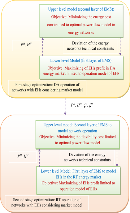
Upper-level formulation (second layer of EMS)
The hour-basis DA operation of the energy networks with EHs is described here. Equations┬Ā(1)-(13) states the problem and includes an objective function so that the minimum energy cost is reached8. Optimal power flow (OPF) equations are presented in Eqs.┬Ā(2) through (13)4,8,9, while power flow equations are presented in Eqs.┬Ā(2) through (7). Equations┬Ā(2)-(5), which also provide the active and reactive power balance of network buses and objects passing across lines, describe the electricity network power flow20,21,22,23. Equations┬Ā(6)ŌĆō(7) give the heating network power flow8. Equations┬Ā(8)ŌĆō(13) are the operation constraints of the energy networks8,9, representing the limitation on bus voltage magnitude, apparent power of distribution lines and substations24,25,26,27, node temperature, and thermal power of heating pipelines and stations.
Lower layer (first layer of EMS)
The goal function, Eq.┬Ā(14), maximizes the EHs profit in electricity and heat energy markets. EHŌĆÖs profit is equal to the total of its revenues in the aforementioned markets. Energy price and power are multiplied to determine revenue in each market28. When power has a positive value, Eq.┬Ā(14) gives EHŌĆÖs revenue; while for its negative value, Eq.┬Ā(14) gives EHŌĆÖs cost. The demand and supply balances for active and heating power are denoted by Eqs. (15)-(16). In these two equations, WT and BU are considered as electrical energy producers29,30,31,32,33, and hydrogen and compressed air storages were utilized as energy storage. BU is equipped with CHP technology9, so in the thermal sector, only BU produces thermal energy. The power of RESs is a parameter34,35,36,37. Also, TES has employed used as an energy store. Equations┬Ā(17)ŌĆō(26) provide the operational model of the ESSs and RESs in EHs. By being equipped with CHP, BU is able to produce electrical and thermal energy at the same time. This is presented in Eq.┬Ā(17), which refers to the amount of thermal power produced by BU based on its active power8. In addition, it should be noted that in the Eqs. (15) and (16), the active power generation by WT and BUs were included as parameters, the amount of which is determined based on weather data. The functioning of EESs including HS and CAES are described in Eqs. (18)ŌĆō(23)7,38. HS has fuel cell (FC), electrolyzer (EL), and hydrogen tank (HT)38. The electrolyzer is active in the HS charging mode and converts the electrical energy into hydrogen39. Then hydrogen is stored in HT. In HS discharge mode, FC is active and it receives hydrogen from HT and converts it into electrical energy38. HS performance model can be seen in Eqs. (18)-(20). The capacity limits of EL and FC are given in constraints (18) and (19), respectively, and the limit on the energy stored in HT is proportional to constraint (20)39. In CAES, a motor stores electrical energy in the form of compressed air in a compressed air tank (CAT) in the CAES charging operation mode. In the discharge mode, CAES also receives a compressed air generator from the CAT and converts it into electrical energy. Following this, the performance model of CAES is in the form of Eqs. (21)ŌĆō(23)7. In Eqs. (21) and (22), the motor and generator capacity limits are included, respectively. In constraint (23), the limitation of energy stored in CAT is considered7. The TES performance model is presented in Eqs. (24)ŌĆō(26)1. Its mathematical model is the same as EES, with the difference that thermal power is used in Eqs. (24)ŌĆō(26). Constraints (24) and (25) state the charge and discharge rate limit40,41,42,43, respectively, then the thermal energy stored in TES is limited based on (26)44. Finally, variables Žæ and ╬╝ represent Lagrange multipliers for equality and inequality equations, respectively.
5-min RT scheduling of EHs in the energy networks (second stage)
Unexpected outcomes in terms of active power may be found when weather conditions affect the output power production of power sources. As a consequence, the supply and demand balance may no longer be maintained for RT operation, indicating inadequate system flexibility9,11. As a solution, the research underlines the utilization of flexibility sources, such as ESSs1. Equations┬Ā(27) minimize the unbalance profit of EHs in DA and RT markets45. This equation presents the flexibility cost. A bi-level optimization framework frames the issue. The upper level objective function is provided in Eq.┬Ā(27), and its constraints include the OPF restrictions on the energy networks are shown in (2)ŌĆō(13). This statement is expressed in (28). Equations┬Ā(29)ŌĆō(30) are used in the lower-level model to determine EHŌĆÖs profit in the RT market. The model provided by Eqs. (14)ŌĆō(15) is analogous to the problem as described in these equations. Finally, it should be noted that minimization of the unbalance between RT and DA operations or flexibility cost based on Eq.┬Ā(27) can achieve 100% flexible EHs in energy networks so that if F3 is zero, it means that flexibility sources including storage systems in EH resolve the oscillation of RES active/heat power in RT operation compared to DA operation. Therefore, in both modes of operation, EHs will always have the same power. This equates to 100% EH adaptability across various networks. As a result, the EHs are more flexible the lower the F3 value. On the other hand, it is anticipated that by decreasing F3, the outcomes of the RT and DA procedures for EH would be comparable.
$$\min \,\,\,\,\,\,F_{3} = \sum\limits_{{\omega \in \Gamma_{S} }} {\sigma_{\omega } \sum\limits_{{\tau^{\prime} \in \Gamma_{{OH^{\prime}}} }} {\sum\limits_{{h \in \Gamma_{H} }} {\left( {\left( {\zeta_{{\tau^{\prime},\omega }}^{E} P_{{h,\tau^{\prime},\omega }}^{H} – \zeta_{{\tau^{\prime},\omega }}^{\prime E} P_{{h,\tau^{\prime},\omega }}^{\prime H} } \right)^{2} + \left( {\zeta_{{\tau^{\prime},\omega }}^{H} H_{{h,\tau^{\prime},\omega }}^{H} – \zeta_{{\tau^{\prime},\omega }}^{\prime H} H_{{h,\tau^{\prime},\omega }}^{\prime H} } \right)^{2} } \right)} } }$$
(27)
Subject to:
$${\text{Constraints }}\,\left( {2} \right) – \left( {{13}} \right)\,{\text{ considering}}\,\tau^{\prime}\,{\text{instead }}\,{\text{of}}\,\tau ,{\text{ and}}\,{\text{ using}}\, \, (.^{\prime}){\text{for}}\,{\text{ parameters }}\,{\text{and}}\,{\text{ variables}}$$
(28)
$$P^{{\prime H}} ,H^{{\prime H}} \in \arg \left\{ {\max \,\,\,\,\,\,F_{4} = \sum\limits_{{\omega \in \Gamma _{S} }} {\sigma _{\omega } \sum\limits_{{\tau ^{\prime} \in \Gamma _{{OH^{\prime}}} }} {\sum\limits_{{h \in \Gamma _{H} }} {\left( {\zeta _{{\tau ^{\prime},\omega }}^{{\prime E}} P_{{h,\tau ,\omega }}^{{\prime H}} + \zeta _{{\tau ^{\prime},\omega }}^{{\prime H}} H_{{h,\tau ,\omega }}^{{\prime H}} } \right)} } } } \right.$$
(29)
Subject to:
$${\text{Constraints }}\,\left( {{15}} \right) – \left( {{26}} \right)\,{\text{ considering}}\,\tau^{\prime}{\text{instead }}\,{\text{of}}\,\tau ,{\text{ and}}\,{\text{ using}}\, \, (.^{\prime}){\text{for}}\,{\text{ parameters }}\,{\text{and}}\,{\text{ variables}}$$
(30)
The frequency of phenomena is determined using prediction data. The pace of the aforementioned occurrences, and eventually the production of renewable energy, does not have a deterministic value and is associated by uncertainty since the forecast of a datum is accompanied by an error. This leads to different day-ahead and real-time operations of a system with renewable resources. Therefore, generation and consumption balance may not be established in real time operation. These conditions are corresponding to the flexibility lack of the system. Therefore, numerous studies, including45, advise using storage devices or demand response strategies in addition to renewable sources. A CHP-based BU is part of an energy hub. The thermal power in a BU is a coefficient of the active power of the BU based on Eq.┬Ā(17). This also leads to a decrease in the flexibility of the energy hub in the thermal sector. Thermal storage is used with BU to address this problem. These substances have the capacity to regulate their thermal power. They will thus be able to increase the thermal part of the energy hubŌĆÖs flexibility. It should be noted that this issue will be comprehensible by providing an adequate formulation that considers the systemŌĆÖs adaptability. Equation┬Ā(27) was used in this instance. If the value of F3 is zero, this equation predicts that real-time and day-ahead operations will provide results that are quite comparable. This issue corresponds to the conditions of high flexibility in the proposed system.
Uncertainty modeling
Uncertainty parameters of the problems (1)-(3) include energy price, ╬ČE, ╬ČH, ╬ŠE, and ╬ŠH, load, PC, QC, and HC; renewable power, PWT and PBU. These uncertainties are modeled in this study in a stochastic framework using the UT method. This method needs fewer executions than Monte Carlo Simulation (MCS) and analytic methods, helping to reduce execution time. Additionally, this approach to modeling uncertainty does not need any assumptions. The UT approach also has the benefit of being able to handle nonlinear transitions8,9 and accurately estimate the probability distribution function (PDF) while simplifying the coding procedure. The stochastic uncertainty parameters are likewise modeled using this way. Parameter n is the dimension of the vector of input uncertainty parameters (U). In this study, nŌĆē=ŌĆē9 is assumed. So, there are 2nŌĆē+ŌĆē1ŌĆē=ŌĆē19 scenarios, with nŌĆē=ŌĆē9. There is no necessity to decrease the number of scenarios in this methodology due to the limited number of scenarios. Further information regarding this methodology can be found in the publication referenced8,9.
The execution step in these issues is minimal. Therefore, the real-time market execution stage in the suggested strategy takes roughly 5 min. As a result, it is essential to find a quick computational solution. The magnitude of the issue is one aspect that influences how long it takes to compute. This problem causes the problemŌĆÖs volume to grow, which may require a lengthy calculation and fall short of the operatorŌĆÖs objectives. The worst-case scenario is the sole possible outcome for this approach. Since this technique has a scenario and produces a robust solution16, it is anticipated that it will take less time to solve the issue than stochastic optimization. However, it should be emphasized that the flexibility of the issue is also taken into account in the suggested approach based on Eq.┬Ā(27). Analyzing various scenarios of renewable energy production is required to determine the precise condition of flexibility. As a result, robust optimization cannot appropriately assess the flexibility issue. This work applies the UT approach to account for the aforementioned circumstances. The stochastic optimization process used here has the fewest possible situations. As a result, it is anticipated to have a short computation time, and using this approach, the level of flexibility may be thoroughly examined.