The SD model was developed to assess the environmental impacts associated with the demolition tools used in building demolitions in Thailand. This model is comprised of eight interlinked sub-models: (1) the number of demolished townhouse units, (2) the percentage of CO2-equivalent (CO2-eq) emissions, (3) the percentage of primary energy consumption, (4) the percentage of noise, (5) the percentage of dust, (6) the percentage of heat, (7) the percentage of vibration, and (8) the overall environmental impact percentage.
The model operates on a detailed causal loop diagram (CLD), as depicted in Fig. 4, which outlines the dynamic interactions of key variables within the demolition process. These interactions are represented through balancing loops that offer a structured approach to understanding and quantifying the environmental impacts. In System Dynamics, CLDs serve as powerful tools for modeling intricate feedback relationships between variables. A (+) sign indicates that both variables move in the same direction, while a (−) sign shows that the variables influence each other opposing directions. Causal loops can be classified as either reinforcing or balancing, contingent upon whether the number of negative links within the system is even or odd. Causal Loop Diagrams (CLDs) encapsulate both reinforcing (positive feedback) and balancing (negative feedback) mechanisms, offering a comprehensive representation of system dynamics. The diagram is further delineated by balancing loops, each denoted by the symbol ‘B,’ which encapsulates distinct interactive processes governing the system’s equilibrium.
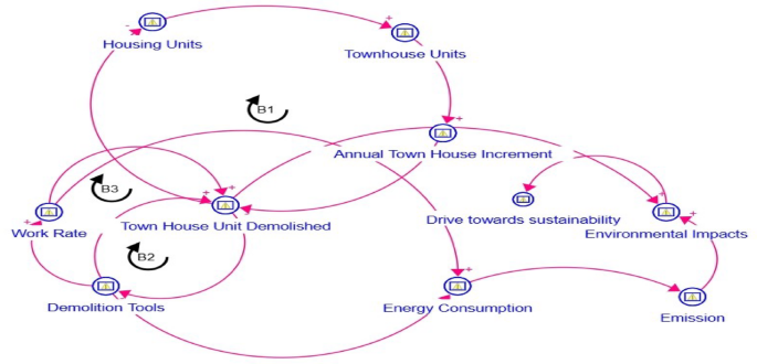
Causal Loop Diagram (CLD) representing key interactions in the demolition process.
These balancing loops represent distinct dynamics. For example:
B1 establishes the interdependence between housing units, the growth in townhouse developments, and subsequent demolition activities. The number of townhouse units is inherently linked to the available housing stock, such that an increase in townhouse units positively influences the annual increment of such structures (+). This, in turn, engenders a proportional relationship between the annual growth of townhouse units and the number of demolitions undertaken. Consequently, as the volume of demolished townhouse units increases, the overall housing stock diminishes (−), thereby illustrating the inherent balancing mechanism that governs these variables.
B2 highlights the interaction between demolition tools and the number of townhouse units demolished. The deployment of a greater number of demolition tools facilitates an accelerated pace of townhouse demolitions. However, as the pool of townhouses designated for demolition progressively contracts over time, the demand for demolition tools correspondingly declines. This cyclical adjustment exemplifies the balancing nature of interactions that regulate these system components.
B3 elucidates the relationship between the work rate and the number of townhouses demolished, which, in turn, modulates the number of tools required. The efficiency of townhouse demolition within a given timeframe is intrinsically tied to the prevailing work rate; as more townhouses are dismantled within a short span, the number of required demolition tools gradually decreases in response to the diminishing stock of structures awaiting removal. This interaction encapsulates the self-regulating characteristics of the system, reinforcing its underlying balancing dynamics.
Thus, the overall model is fundamentally grounded in the detailed CLD, providing a comprehensive view of the interconnected elements governing the demolition process.
Sub-model for the number of demolished townhouses
In 2022, Bangkok recorded a total of 3.2 million housing units, reflecting an annual growth rate of 2.56%3,4. Among these, townhouses accounted for approximately 51%26, with an estimated 10% of new construction permits linked to townhouse demolitions. Townhouses are generally classified into three size categories: small, medium, and large5. Notably, the proportion of small-sized townhouses has been growing at an annual rate of 6.4%, while larger townhouses have seen a decline of 8.5% per year26. These opposing trends contribute to divergent demolition rates across different townhouse sizes, significantly influencing the housing landscape in Bangkok.
$$\:\text{N}\text{T}\text{D}=\text{S}\text{T}\text{D}+\text{M}\text{T}\text{D}+\text{L}\text{T}\text{D}$$
(1)
.
The environmental impact of demolition activities depends on several factors, including the number and size of townhouses being demolished, as indicated in Eq. (1), as well as the specific combination of tools employed. Larger townhouses typically require prolonged work durations with heavy machinery, such as excavators, compared to medium or small-sized units. This extended operational time not only increases primary energy consumption, but also intensifies the generation of dust, noise, and vibration, resulting in a heightened environmental footprint. Therefore, the scale of demolition and the selection of tools are critical in determining the magnitude of environmental disturbances.
Sub-model for the proportional impact of primary energy consumption
The calculation of primary energy consumption for the tools used in Combination 1 (excavators, jackhammers, and flame cutters) is based on several factors: power ratings, energy conversion coefficients, work rates, operating hours, and the number of tools employed. For example, a diesel-powered excavator with a power rating of 210 kW17 and an energy conversion factor of 0.086 kgoe/kWh17 is responsible for 50% of the work rate in Combination 1. This is compared to electric Jackhammers, which have a power rating of 2.2 kW17 and an energy conversion factor of 1.952 kgoe/Kwh17. Flame cutters, rated at 1.5 kW17 with the same energy conversion, operate at 10% of the total work time. Small, medium, and large-sized townhouses each require one excavator, along with two, four, and six jackhammers, and two, two, and four flame cutters, respectively. For small, medium, and large townhouses, with total work times of 64, 96, and 128 hours17the respective primary energy consumptions are calculated in Eqs. (2)–(4).
The overall primary energy consumption is obtained by aggregating the energy consumption of all tools in Combination 1. This total is then adjusted to calculate the percentage contribution of primary energy consumption for this specific tool combination.
$$\:\text{P}\text{E}\text{E}1=210\:\times\:0.086\:\times\:0.5\:\left[\left(\text{S}\text{T}\text{D}\:\times\:64\right)+\left(\text{M}\text{T}\text{D}\:\times\:96\right)+\left(\text{L}\text{T}\text{D}\:\times\:128\right)\right]$$
(2)
$$\:\text{P}\text{E}\text{J}1=2.2\:\times\:1.952\:\times\:[\left(\text{S}\text{T}\text{D}\:\times\:2\:\times\:64\right)+\left(\text{M}\text{T}\text{D}\:\times\:4\:\times\:96\right)+\left(\text{L}\text{T}\text{D}\:\times\:6\:\times\:128\right)]$$
(3)
$$\:\text{P}\text{E}\text{F}1=1.5\:\times\:1.952\:\times\:0.1\left[\left(\text{S}\text{T}\text{D}\:\times\:64\right)+\left(\text{M}\text{T}\text{D}\:\times\:2\:\times\:96\right)+\left(\text{L}\text{T}\text{D}\:\times\:6\:\times\:128\right)\right]$$
(4)
.
The calculated primary energy consumption for Combination is compared with the consumption values for the remaining combinations. The combination with the highest consumption is assigned a baseline of 100%, representing the most significant environmental impact among the four combinations. The primary energy consumption percentages for the other combinations are then adjusted in proportion, reflecting their relatively lower energy usage (please refer to Eqs. (5) and (6)).
$$\:\text{M}\text{A}\text{X}\text{T}\text{P}\text{E}=\text{M}\text{A}\text{X}\left(\text{T}\text{P}\text{E}1,\:\text{T}\text{P}\text{E}2,\text{T}\text{P}\text{E}3,\:\text{T}\text{P}\text{E}4\right)$$
(5)
$$\:\text{T}\text{P}\text{E}1\text{N}=\text{T}\text{P}\text{E}1/\text{M}\text{A}\text{X}\text{T}\text{P}\text{E}\:\:\times\:100$$
(6)
.
Sub-model for the percentage impact of CO2-eq emissions
The CO2-eq emissions for each tool are estimated by multiplying their primary energy consumption by conversion factors, the number of tools used, work rates, and the demolition duration. According to the Ministry of Energy’s Energy Policy and Planning Office66the CO2-eq emission for electricity-powered demolition equipment is calculated using a conversion factor of 0.495 kg CO2-eq/kWh7, while the factor for diesel-powered excavators 2.025 kgCO2eq/kWh14. Equations (7)–(9) show examples of the CO2-eq emissions (in kg CO2-eq) for Combination 1 (diesel-powered excavators, electric jackhammers, and flame cutters). The individual CO2-eq emissions are aggregated to calculate the total for Combination 1, which is then adjusted to reflect the corresponding dust impact percentages for this tool combination.
$$\:{\text{C}\text{O}}_{2-\text{e}\text{q}}\text{E}1=2.025\:\times\:\text{P}\text{E}\text{E}1\:\times\:0.5\left[\left(\text{S}\text{T}\text{D}\:\times\:64\right)+\left(\text{M}\text{T}\text{D}\:\times\:96\right)+\left(\text{L}\text{T}\text{D}\:\times\:128\right)\right]$$
(7)
$$\:{\text{C}\text{O}}_{2-\text{e}\text{q}}\text{J}1=0.495\:\times\:\:\text{P}\text{E}\text{J}1\:\times\:[\left(\text{S}\text{T}\text{D}\:\times\:2\:\times\:64\right)+\left(\text{M}\text{T}\text{D}\:\times\:4\:\times\:96\right)+\left(\text{L}\text{T}\text{D}\:\times\:6\:\times\:128\right)]$$
(8)
$$\:{\text{C}\text{O}}_{2-\text{e}\text{q}}\text{F}1=\:0.495\:\times\:\:\text{P}\text{E}\text{F}1\:\times\:[\left(\text{S}\text{T}\text{D}\:\times\:2\:\times\:64\right)+\left(\text{M}\text{T}\text{D}\:\times\:2\:\times\:96\right)+\left(\text{L}\text{T}\text{D}\times\:4\:\times\:128\right)]$$
(9)
.
Sub-model for the percentage impact of noise
The noise percentage for each demolition tool within a combination is derived from several interrelated factors: noise levels, townhouse sizes, work rates, the number of tools used, and the duration of operations. Specifically, Eqs. (10) and (11) demonstrate the calculation of noise levels for Combination 1, accounting for emissions from excavators and jackhammers but excluding flame cutters, as they do not contribute to noise pollution. The cumulative noise from these tools is aggregated to determine the total noise output, which is then normalized and adjusted to calculate the noise percentage for this combination.
$$\:\text{N}\text{E}1=112\:\times\:0.5[\left(\text{S}\text{T}\text{D}\:\times\:64\right)+\left(\text{M}\text{T}\text{D}\:\times\:96\right)+\left(\text{L}\text{T}\text{D}\:\times\:128\right)]$$
(10)
$$\:\text{N}\text{J}1=113\:\times\:0.4\left[\left(\text{S}\text{T}\text{D}\:\times\:2\:\times\:64\right)+\left(\text{M}\text{T}\text{D}\:\times\:4\times\:\:96\right)+\left(\text{L}\text{T}\text{D}\:\times\:6\times\:128\right)\right]$$
(11)
.
Sub-model for the percentage impact of dust
Dust emissions from Combination 1, produced by the excavator and jackhammer (as flame cutters does not generate dust), are determined by multiplying the arithmetic mean of respirable dust produced by these tools—1.4 mg/m³ for the excavator and 3.4 mg/m³ for the jackhammer—by their respective work rates, operating hours, and the number of tools used. The dust output from both tools is then aggregated to determine the total dust emissions for Combination 1, which is subsequently adjusted to reflect the dust percentages for this tool combination.
$$\:\text{D}\text{E}1=1.4\times\:0.5\left[\left(\text{S}\text{T}\text{D}\:\times\:64\right)+\left(\text{M}\text{T}\text{D}\:\times\:96\right)+\left(\text{L}\text{T}\text{D}\:\times\:128\right)\right]$$
(12)
$$\:\text{D}\text{J}1=3.4\:\times\:0.4\left[\left(\text{S}\text{T}\text{D}\:\times\:2\times\:64\right)+\left(\text{M}\text{T}\text{D}\:\times\:4\:\times\:96\right)+\left(\text{L}\text{T}\text{D}\:\times\:6\:\times\:128\right)\right]$$
(13)
.
Sub-model for the percentage impact of heat
In Combination 1, heat is generated solely by the flame cutters, which operate at 850 kJ. Neither the excavator nor the jackhammer contributes to heat production (see Eq. 14). The calculation of heat output considers the number of flame cutters used, their work rates, and the number and size of townhouses being demolished, providing a detailed assessment of heat generation in this tool combination.
$$\:\text{H}\text{F}1=850\:\times\:0.1\left[\left(\text{S}\text{T}\text{D}\:\times\:2\:\times\:64\right)+\left(\text{M}\text{T}\text{D}\:\times\:2\:\times\:96\right)+\left(\text{L}\text{T}\text{D}\:\times\:4\times\:128\right)\right]$$
(14)
.
Sub-model for the percentage impact of vibration
In Combination 1, vibrations generated by both the excavator and the jackhammers, as outlined in Eqs. (15) and (16). The vibration output from these tools is aggregated to determine the total vibration produced. This total is then adjusted to calculate the vibration percentage for this combination, providing a comprehensive assessment of the vibration impact associated with this tool combination.
$$\:\text{V}\text{E}1=2.9\:\times\:0.5\left[\left(\text{S}\text{T}\text{D}\:\times\:64\right)+\left(\text{M}\text{T}\text{D}\:\times\:96\right)+\left(\text{L}\text{T}\text{D}\:\times\:128\right)\right]$$
(15)
$$\:\text{V}\text{J}1=0.9\times\:0.4\left[\left(\text{S}\text{T}\text{D}\:\times\:2\times\:64\right)+\left(\text{M}\text{T}\text{D}\:\times\:4\:\times\:96\right)+\left(\text{L}\text{T}\text{D}\:\times\:6\:\times\:128\right)\right]$$
(16)
.
Sub-model for the overall environmental impact percentage
The calculated percentages for the six environmental impacts are weighted according to their assigned importance (see Table 3). For example, the percentages for primary energy consumption and CO2-eq emissions are multiplied by their respective weights of 6.3 and 20.8. The weighted percentages for all six environmental impacts—primary energy consumption, CO2-eq emissions, noise, dust, heat, and vibration—are aggregated and divided by the total importance weight of 34.2 (as shown in Table 3) to determine the overall environmental impact percentage. Equation (1) demonstrates the final impact percentage calculation for Combination 1.
$$\:\text{O}\text{E}\text{I}\text{C}1=(\left(\text{T}\text{P}\text{E}1\text{N}\:\times\:6.3\right)+\left({\text{C}\text{O}}_{2-\text{e}\text{q}}1\text{N}\times\:20.8\right)+\left(\text{T}\text{N}1\text{N}\:\times\:2.3\right)+\left(\text{T}\text{D}1\text{N}\times\:2\right)+\left(\text{T}\text{H}\text{I}\text{N}\times\:1.8\right)+\left(\text{T}\text{V}\text{I}\text{N}\:\times\:1\right))/34.2$$
(17)
.
Machine learning (ML) system development
Given the integration of SD modelling with the RF algorithm—an advanced supervised machine learning (ML) approach—the dataset, comprising multiple combinations of demolition tools and their associated environmental impacts, was extracted from the comprehensive SD model and carefully structured for subsequent RF analysis. This integration enables a robust evaluation of the environmental consequences associated with each demolition tool combination.
The first phase of the process involved loading the environmental impact dataset and performing essential pre-processing steps, such as splitting the data into features (input variables) and the target (output variable). The dataset was then partitioned into training and testing subsets, adhering to an 80–20 split. This ratio ensures that a substantial portion of the data is used for training, while retaining sufficient data for testing and validation—especially important given the dataset size57,67.
Following data preparation, the RandomForestRegressor was initialized with carefully selected parameters. The n_estimators parameter was set to 100, based on evidence suggesting that a higher number of trees enhances both performance and stability68,69. The maximum depth of the trees was set to the default value of 5 to avoid both under- and over-fitting70. A random state of 42 was applied to ensure reproducibility. The RF model was then trained using the training dataset, constructing multiple decision trees, each based on a random subset of both the data and its features.
Once training was completed, predictions were generated for both the training and testing datasets to assess potential overfitting and generalization, respectively. The model’s performance was evaluated using standard regression metrics, including Mean Squared Error (MSE), R-squared (R2) score, and the R-score.
Additionally, the RF algorithm performed a feature importance analysis to assess the contribution of each feature—representing the environmental impacts associated with different combinations of demolition tools—to the model’s overall predictive accuracy. This was accomplished by quantifying the influence of each feature on the model’s performance. To further enhance performance, the model underwent hyperparameter tuning, focusing on key parameters such as n_estimators, max_depth, and min_samples_split. This optimisation was carried out using the Grid Search technique, which systematically explores various parameter combinations to identify the most effective configuration60.
It is important to underscore that the RF algorithm is a powerful tool for both classification and regression. In the context of this study, the RF algorithm leverages the precision of SD modelling alongside the predictive capabilities of multiple decision trees to deliver results that are both accurate and robust. The key steps in implementing the algorithm include data extraction and preparation, model initialisation, prediction generation, performance evaluation, feature importance analysis, and model tuning, all of which contribute to the efficacy of the RF in tackling complex predictive tasks.