The performance of individual regression models, which includes XGBoost, CatBoost, Random Forest, Gradient Boosting, Extra Trees, and AdaBoost, was assessed with respect to standard statistical measures such as R², adjusted R², MAE, and RMSE. Results for the different trials conducted on these models are compiled in Table 9 S (Attached in the Supplementary file). In terms of the evaluated algorithms, CatBoost achieved an R² of 0.9894, and Gradient Boosting achieved an R² of 0.9907, both showing superior accuracy among the individual models alongside lower RMSE and MAE than Random Forest and Gradient Boosting. While Extra Trees and AdaBoost performed reasonably well, their predictive performance was notably less. These differences in performance can be explained by the underlying differences in the algorithms, particularly CatBoost’s adeptness at utilizing categorical features and XGBoost’s ability to exploit complex interactions and nonlinear relationships among features within environmental data sets.
Further analyses on convergence and stability were performed using the training loss curves Fig. 4a–d., which showed the RMSE drops during training iterations. These plots show that both CatBoost and XGBoost had better final predictive performance, but they also converged faster, which indicates better efficiency. This illustrates once more how much algorithm choice and hyperparameter optimization matter and proves that the methods based on gradient-boosted decision trees are effective for complex environmental modeling problems. Various training convergence (RMSE loss curves) results are shown below.
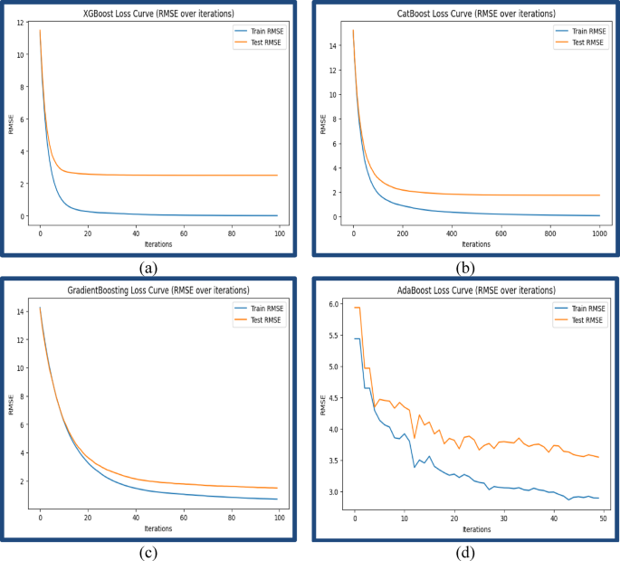
Model training performance based on loss curves (RMSE vs. iterations) for ensemble regressors. (a) XGBoost loss curve, (b) CatBoost loss curve, (c) Gradient Boosting loss curve, and (d) AdaBoost loss curve.
The R² scores and RMSE provided in Table 10 S (Attached in the Supplementary file) were utilized to evaluate the predictive performance of the different models. For some of the models, such as XGBoost, CatBoost, and Gradient Boosting, which support iterative training, training loss curves were also produced to assess convergence reliability during model training for additional insights into predictive stability and convergence. The training loss curves depicted in Fig. 4 (a–d) illustrate the RMSE convergence behavior for each ensemble regressor. CatBoost and XGBoost not only achieved the lowest final RMSE values but also demonstrated rapid and stable convergence during training, indicating strong learning efficiency and lower overfitting risk. Gradient Boosting, while accurate, showed slower convergence, and AdaBoost displayed higher final RMSE and fluctuation, reflecting its relative sensitivity to noisy features. These trends reinforce the suitability of gradient-boosted frameworks, especially CatBoost and XGBoost, for complex water quality datasets where interactions and non-linearities are prominent. This convergence analysis further supports the decision to include these models in the final stacked ensemble.
Model performance
The stacking ensemble, where the meta-learner is a Linear Regression model integrating predictions of base models, performed considerably better than the individual regressors. As previously stated with R², adjusted R², MAE, and RMSE, the ensemble’s predictive performance was better than the single model approaches, with an astounding R² score nearing 0.995 and an RMSE around 1.07, as highlighted particularly in Table 11 S (Attached in Supplementary file). These great changes were the results of the ensemble stacking model’s ability to diminish the bias and variance produced by individual models by efficiently utilizing the predictions of all base models. Ensemble models such as XGBoost, CatBoost, and Gradient Boosting provide robustness by combining predictions from multiple weak learners and consequently improving predictions by reducing bias and variance. Ensuring high prediction accuracy is valuable when building predictive models on environmental datasets, which are inherently non-linear and often noisy data. Ensemble models handle multicollinearity, feature interaction, and missing predictor data better than many methods, also improving their reliability and generalization across future datasets. In this study, the stacked ensemble framework produced improvements over individual models on key statistical measures of fit, which showed that the stacked ensemble model produced robustness for modeling WQI in real time and, hence, scalable predictions. The stacking ensemble structure in Fig. 3 demonstrates how the outputs of the base regressors are used as inputs into the linear regression meta-learner, illustrating the use of the base models for the improvement of predictive accuracy. Through a fivefold CV, the predictive accuracy and robustness of the predictors were tested thoroughly, demonstrating the predictive consistency and generalization of the stacking ensemble. This portrays stacking ensembles as powerful models for environmental predictive analytics, proving traditional models to be inefficient. As illustrated in Table 2, which captures the analytical results of different predictive models, the Stacked Regression Ensemble model’s performance was evaluated using standard statistical metrics (R², Adjusted R², MAE, RMSE) and found to outperform other models consistently. Table 2 marks the regimented analysis of evaluation results where the predictive strength of the ensemble model bested that of individual models.
The stacked ensemble model also performed well relative to the individual top models examined, achieving an R² of 0.9952 and an RMSE of 1.0704 (Table 11 S). As shown in Table 11 S of the Supplementary Material, the stacked ensemble outperformed all individual regressors across R², Adjusted R², MAE, and RMSE, demonstrating superior generalization and predictive strength. In contrast, the best individual models, Gradient Boosting and CatBoost, had R² values of 0.9907 (RMSE = 1.4898) and 0.9894 (RMSE = 1.5905), respectively. This demonstrates the value of using stack ensemble models to generate predictions that are both more accurate and more stable. Every regression-based ML model included in the stacking ensemble framework shows different unique advantages and challenges, as each impacts predictive performance, computational efficiency, and practical utility. These characteristics are presented in Table 3, providing practical information necessary for the optimal selection of highly accurate predictive models depending on the datasets, the associated complexity, available computational resources, and precision requirements. Unlike previous studies that employed individual models or limited ensembles, our stacked regression ensemble integrated with SHAP-based explainability not only achieved the highest predictive accuracy (R² = 0.9952, RMSE = 1.0704) but also resolved the black-box challenge, offering both precision and interpretability in a unified framework (Table 3).
Model interpretability using SHAP analysis
The SHAP analysis was carried out to improve predictive transparency (SHAP) and explains how prediction features at the model level are usually interpreted by employing a game-theoretic approach. Global and local model interpretability were systematically examined using SHAP’s TreeExplainer with XGBoost models. Numerous visualizations of SHAP values were created, including the SHAP parameter value summary plot (Fig. 5a), dependence plot (Fig. 5b), individual SHAP value prediction force plot (Fig. 5c), and distribution of SHAP values for each parameter (Fig. 5 d). Depicting the distribution of contribution parameters, which demonstrated the effect predictive parameters had on predictive outcomes. Stakeholders enhanced predictive model transparency, interpretability, and confidence due to the SHAP visualization framework.
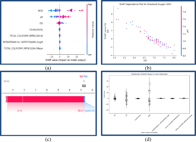
SHAP-based model interpretability visualizations. (a) SHAP summary plot illustrating the overall influence of each feature on model output. (b) SHAP dependence plot highlighting interactions between individual features and their corresponding SHAP values. (c) SHAP force plot showing localized, sample-specific explanations of individual predictions. (d) SHAP plot representing the distribution and variability of feature contributions across all observations. SHAP values were calculated at the base learner level using TreeExplainer, and they were summarized for the meta-learner using a model-agnostic SHAP approach to increase the interpretability of the potential-based ensemble framework. This allowed for the global and local explanation of the model’s predictions, as outlined in the following section.
Feature importance and interpretability through SHAP analysis
Interpretability is crucial for enabling the responsible use of ML models for environmental monitoring, especially for sensitive purposes like compliance trends that pertain to regulated thresholds, risk evaluation, or health impact assessment. While regression models provide more granular, continuous forecasts of WQI and are suited for trend prediction, classification models still hold practical significance. They are effective in communicating categorical water quality status (e.g., Excellent, Poor) and are often used in regulatory decision-making based on defined thresholds. Thus, a hybrid approach can sometimes be beneficial depending on end-user requirements. Figure 5 (a–d) provides the multi-level SHAP analysis: (a) the feature-wise summary importance, (b) the dependence on WQI prediction on DO with pH interaction, (c) the force plot for an individual prediction, (d) SHAP value distributions for all samples. Together, these visual figures provide global and local interpretability of the model’s reasoning with further justification for BOD, DO, pH, and conductivity as key determinants of WQI. In this work, we applied SHAP, i.e., an explainable AI (XAI) method that draws on cooperative game theory to rationalize its predictions to our stacked regression ensemble framework to make the models more interpretable. SHAP values quantify the amount of each feature’s contribution to a given prediction, quantifying whether the feature was helpful or detrimental to achieving the expected outcome. This was especially useful because our model was highly predictive (R² = 0.9952, RMSE = 1.0704), enabling us to deconstruct intricate behavioral patterns into simpler, actionable insights at the feature level. To ensure broader interpretability of the outcome, four SHAP-based visualization tools were used: summary plots, dependence plots, force plots, and parameter-wise SHAP value distributions. Each of them had a different analytical focus, including determining the main contributors for the WQI, describing their influences together with other variables, explicating particular outcomes, and evaluating the stability and reliance of that feature throughout the data. The range shows that higher BOD concentrations usually conveyed negative SHAP values (lower WQI predictions), while lower concentrations of BOD provided positive SHAP contributions, which was expected from an environmental aspect, noting organic pollution and oxygen demand. The SHAP summary plot (Fig. 4a) showed the clear ranking of features and their importance based on the value and sign of SHAP values. This ranking not only reflects statistical importance but also aligns well with ecological understanding, confirming that the model has successfully internalized key environmental interactions such as organic loading from BOD and oxygen replenishment from DO. In terms of impact on model predictions, BOD had the greatest effect, with SHAP values ranging from − 12 to + 24, so it was the most important negative contributor to WQI. This is because high BOD values are well known to indicate organic pollution and low availability of DO, thus degrading water quality. This environmental rule was learned correctly by the ensemble model and confirmed with SHAP analysis. pH was next in the rank order and exhibited approximately SHAP contributions, ranging from − 10 to just under + 20, confirming its strong but context-sensitive influence on WQI prediction. Higher pH values (> 7.5) were largely beneficial predictors of WQI, though negative SHAP values were noted. The negative values appeared in samples with high pH and low DO and/or high BOD, which presumably is due to interactions that the algorithm successfully identified. This phenomenon highlights the model’s ability to capture complex dependencies in the environment. Since pH is an important determinant of chemical equilibrium and biological activity in water, its role was context-sensitive and impacted other parameters that determine DO solubility and nutrients in the water body. A key ecological health indicator, DO, positively influenced the model consistently (SHAP ≈ −8 to + 16). In some instances, marginally negative SHAP values for high levels of DO were observed. This is likely due to interactions with other parameters like high pH or low BOD levels, where the contributions of DO to WQI may have attenuated. However, the salient pattern suggests that DO had a positive impact on water quality. Higher DO levels resulted in increased WQI predictions, which are indicative of supporting life in water and thus reflect a positive role in sustaining aquatic organisms. Conductivity, which measures ionic concentrations are due to dissolved salts and industrial pollutants, also meaningfully contributes (SHAP ≈ − 6 to + 9), particularly in moderately disturbed environments. Conductivity is a measure of dissolved ionic species, which generally result from industrial discharge and runoff from agricultural and urban sources. In moderately disturbed systems, where ionic loads exhibit fluctuations without significant variances, conductivity can serve as a reliable indicator of human impacts. The SHAP analysis indicates it contributes to WQI prediction between approximately − 6 and + 9, suggesting a modest and context-dependent contribution. This range suggests that conductivity captures short-term and transient changes in water chemistry across habitats with different but relatively stable ionic backgrounds. On the contrary, parameters like Nitrate-Nitrite, Fecal Coliform, and Total Coliform had low SHAP values (typically ± 3 or less), indicating minimal impact on the model’s decision-making. These low correlation values are consistent with the SHAP analysis, which also indicated the minimal influence of Fecal and Total Coliforms on WQI prediction, possibly due to their sparse representation and varying dynamics compared to BOD. The SHAP results are consistent with the weak statistical relationship we observed between Conductivity and Total Coliform (r ≈ 0.14) in Sect. 3.2, which reinforces their separation in terms of pollution profiles (i.e., Conductivity related to ions, Total Coliform to fecal contamination). Conductivity had an overall moderate contribution towards WQIs, while Total Coliform had limited statistical evidence due to its limited occurrences and wide distribution, resulting in a minor contribution of SHAP impact. This is likely the result of a lack of range/data value diversity or too much correlation with other metrics/model features, rendering them useless during model training. To analyze how these features are interrelated and their impact on the prediction on a continuous scale, the SHAP value for DO was analyzed using a SHAP dependence plot (Fig. 4b). This visualization shows how SHAP values capture the DO values, and their contributions concerning SHAP values provide an increasing positive contribution from 5.0 to 8.0 mg/L of DO concentration. Importantly, the pH color gradient demonstrates profound second-order interaction: higher pH (> 7.5) samples exhibited steeper positive SHAP responses, which underscored the strong synergistic interaction of DO and pH in enhancing water quality. While the dependence plot for DO provides the interaction interpretation associated with a SHAP value as it is so important ecologically, there was a wider variation of SHAP values (–8 to + 16) for this variable, enabling an effective visualization for only this variable, and BOD and pH were examined in different SHAP visualizations (Fig. 5a and d). In future versions of this analytical framework, we may put this level of individual data interpretation up in individual dependence plots for BOD and pH as well. Such views can be understood using the reasoning of chemistry and biology because the solubility and the oxygen uptake are greater for the neutral to mildly alkaline conditions. The ability of SHAP to demonstrate these subtleties of interactions reflects the interdependence of systems working at different dimensions, making the analysis of complex environmental systems effective. Besides understanding these global relationships, the SHAP force plot (Fig. 4c) analyzed the explanations for some parameters to create a singular prediction, in this case, a WQI value of 96.32. For this particular example, pH equalling 7.8 was modeled as a strong positive driver, while BOD (4.9 mg/L) vastly dampened the expectation. Conductivity (81 µS/cm) added a minor yet perceptible negative impact. Such detail allows different stakeholders, including environmental engineers and policy analysts, to follow the reasoning why a certain assessment was done so that AI predictions can be explained and audited. This functionality is crucial for the real-time diagnosis of anomalies requiring intervention, as observed in the cases of IoT-enabled water quality monitoring stations. In order to understand how consistently each feature impacted predictions over the whole dataset, we analyzed the distribution of overall SHAP values for each parameter (Fig. 4 d). These plots captured the range, mean, and concentration of features’ contributions. BOD, being most important with great context-dependent variability, also had the widest SHAP value range (–12 to + 24). This wide span suggests that while BOD is consistently influential, its impact magnitude varies across different water samples, which may be due to differences in pollution sources, ecosystem buffering capacity, or both. DO and pH had greater concentrations around the ± 10 mark, meaning that they were less stable and more uniform throughout all locations and seasons in the dataset. On the other hand, Conductivity had a smaller range (± 6), meaning that it had a moderate impact on WQI predictions but was less variable. Nitrate-nitrite and the microbial indicators did have a more compact, zero-centered SHAP distribution, reinforcing their minimal role rationale for this model’s predictive logic. The minimal contribution is likely due to the following two primary reasons: (i) there was low variability and a skewed distribution in the data, particularly for coliforms with > 67% missing data, as well as high outlier values; and (ii) there was little correlation with other important physicochemical indicators (specifically, DO and BOD) in the correlation matrix (see Sect. 3.2). Thus, the model gave less importance to these features while training. The SHAP framework could also confirm this influence because there was a limited range of SHAP values (generally within the ± 3 range) for coliforms, which suggested limited influence on WQI value prediction. Like the other parameters, coliforms had some regulatory relevance, but their limited statistical and predictive signal in this data limited the weight in the ensemble model accordingly. These trends mean that the model accurately distinguishes between high-impact variables to incorporate into the model and low-signal features, resulting in overfitting and noise amplification. Moreover, the persistent SHAP distributions of DO, pH, and conductivity across samples suggest the possibility of generalizing this model to new datasets with similar ecological baselines. These findings, from a systems management point of view, elaborate on the practicality of embedding SHAP-enhanced AI models in water governance frameworks. This approach facilitates stakeholder confidence, regulatory clarity, and smart actions through its interpretive power and high accuracy, aiding governance and policymaking at every level. The SHAP-interpretability feature is helpful in stepping up the strategic command of AI in the environment, from guiding regional pollution control policies down to providing local monitoring stations with programmable real-time alert systems. These findings, from a systems management point of view, elaborate on the practicality of embedding SHAP-enhanced AI models in water governance frameworks. This approach facilitates stakeholder confidence, regulatory clarity, and smart actions through its interpretive power and high accuracy, aiding governance and policymaking at every level. The SHAP-interpretability feature is helpful in stepping up the strategic command of AI in the environment, from guiding regional pollution control policies down to providing local monitoring stations with programmable real-time alert systems. The SHAP-based interpretability demonstrated that the model picked up recognized environmental relationships; for example, high BOD has a negative effect on WQI, and DO has a positive effect, confirming the model’s consistency with established ecological principles.
Limitations and future directions
Despite the significant methodological advancements in this study, there are certain limitations to acknowledge. Most of the data came from just a handful of river sites in India, so the model might not work well in places with different weather or geography. It must be tested using data from various regions to see how well it works in other areas. The stacking ensemble method used in this study showed good potential, but its performance depends on picking the right models and fine-tuning them properly. Future work should look into how sensitive the results are to these choices, try more tuning, and test the model on completely new datasets to ensure reliability. This study highlights the strong potential of the stacking ensemble method, emphasizing the importance of careful model selection and tuning for optimal performance. Future work should explore the model’s sensitivity to these factors, enhance tuning strategies, and validate results on diverse datasets. The real-time implementation of the framework is practical and scalable, and it connects to IoT-enabled sensor networks. The proposed essential input parameters (DO, BOD, pH, conductivity, nitrate, and coliforms) can be readily gathered using commercially available multi-parameter water quality sensors. These sensors can provide continuous data streams to feed into the trained ensemble model for real-time WQI predictions. Consequently, models can enable automated early warning systems, regulatory alerts, and adaptive management plans. However, real-time implementation will also rely on calibration, environmental noise, and data integrity. As a critical future research direction, aspects of the framework could be developed using digital twins and cloud-based processing of observations and model outputs to facilitate accurate and timely decision-making in adaptive triage of smart water quality monitoring networks. Furthermore, implementing sophisticated deep learning models such as LSTM and transformers may increase forecast accuracy by capturing complicated spatiotemporal patterns, making the system more suitable for large-scale environmental applications.