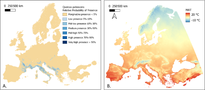
The European Tree Atlas collates and analyses forest tree species occurrence data from various sources across European countries. The results are used to produce a series of species distribution maps. The model-derived maps produced are for Relative-probability of presence (Fig. 1A) and Maximum Habitat Suitability (de Rigo et al., 2016). The latter highlights areas across Europe where tree species could potentially survive, based on many climatic variables. This would theoretically allow us to verify for a given location which species are more likely to survive. However, the lack of some key species for which this data is unavailable and the lack of a temporal dimension that doesn’t allow an assessment of suitability in future climatic conditions, limits its use for species selection based on climate change vulnerability, hence the motivation for the analysis proposed here.
The reason for using such probability of presence data compared to occurrence data, falls on the fact that the latter offers an often biased distribution that requires modelling for it to be a closer representation of the species true distribution, as presence or absence cannot be assumed where occurrence is not recorded27,28. One of the aims of the European Tree Atlas was to eliminate as much as possible the limitations due to the sparse and incomplete nature of multi-source occurrence data. Furthermore, being probability of presence data, it provides information of not only presences, but also absences, useful for quantifying a species climatic niche.
European climate
The ClimateEU project provides gridded climate data for Europe through aggregation and enhancement of data from several publicly and not publicly available databases. It provides monthly, annual, decadal, and 30-year normal climate data for the years 1901 to 2019 as well as multi-model (CIMP5) climate change projections, which are not used here. Gridded bioclimatic variable data is available at a resolution of 1 km2 allowing its use for spatial data analysis (Fig. 1B)29.
In order to check the robustness of our results, we also use an alternative climate gridded dataset, WorldClim version 2.1. Thissimilarly offers gridded bioclimatic variables for the global land surface, averaged over the 1970–2000 period, at an approximate resolution of 1 km2. This gridded product was generated through the interpolation of weather station data from a dataset comprising up to 60,000 weather stations, in conjunction with satellite data30. Climate EU provides a higher quality dataset, as it uses data from WorldClim combining it with data from other packages and processing it to make it more relevant to Europe.
The choice of using publicly available datasets is aimed at enhancing the reproducibility of our work, and it is an improvement with respect to our main referenced previous work17which used a commercial software to produce the gridded climate dataset (ANUCLIM).
Pilot area
L’Aquila is a medium-size city with a population of approximately 70,000, located in the region of Abruzzo in Central Italy. It is located in the Middle Aterno Valley, which extends from north-west to south-east between the Gran Sasso Massif to the North, the largest and highest mountain massif of the Apennines mountain range, and the Velino-Sirente Massif to the South. The altitude of the main urbanized are is between 650 and 720 m a.s.l. One proposed pilot forest site is located in the western part of the city (Fig. 2), characterized mostly by the presence of industrial and commercial warehouses, residential neighbourhoods and sparse unmanaged patches of vegetation.
The composition of the native flora of the surrounding area, because of its mountainous terrain, is primarily defined by altitudinal gradients. Natural and semi-natural areas tend to be well preserved with most of them falling inside protected national parks. Agricultural habitats (pastures and crops) are concentrated in the flats closest to the city’s urban area, while woodland becomes the primary habitat type as the elevation gradient changes. Two main types of woodlands are mostly observed: native Quercus dominated natural and semi-natural deciduous forests and locally non-native Pinus nigra coniferous plantations32. These two main forest types are often merged together, particularly at higher elevations. The city’s climate is classified as continental temperate without dry season and warm summer or Cfb according to the Köppen-Geiger climate classification33. The city’s Mean Annual Temperature is 12.5 °C (1991–2020) and has ranged from 10.7 °C to 13.4 °C in the years 1974 to 2022. The Mean Annual Precipitation is 650 mm/year (1991–2020) and has ranged 440–951 mm/year in 1974–2022. The highest temperatures occur in August with a mean maximum temperature of 31 °C. Lowest temperatures tend to occur mostly in January with the mean minimum temperature being − 2.0 °C.
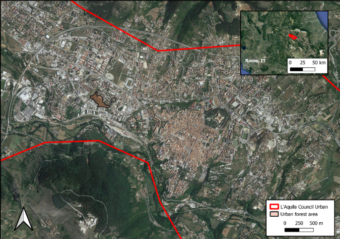
Satellite image of the city of L’Aquila, the location of the proposed urban forest and the city’s geographical collocation. Map produced with QGIS31.
Local climate observations
A long-term time series of daily temperature and precipitation from 1974 to 2022 is taken from previous work33. The dataset was carefully checked for data quality and has been subject to a homogenization procedure, in order to correct the unavoidable discontinuities (e.g. due to instrumental updates or site relocation) affecting multi-decadal weather station observations. The corrected time series show an increasing trend of temperature in the recent decades, in the order of about + 6 °C/century for daily maximum temperature, + 4 °C/century for daily minimum temperature, while for precipitation the trend is less clear.
We use this local climate dataset also to bias correct future climate projections for the scenarios SSP 126 and SSP 585. The method used for bias correction is the ISIMIP3BASD v1.034, which is a quantile-based adjustment method for climate projections developed for the Inter-Sectoral Model Intercomparison Project (ISIMIP) that is aimed at preserving trends in the original projection across quantiles, in order to have a robust correction for both central and extreme values. The correction for precipitation is multiplicative, while that for temperature is additive. In a recent intercomparison of bias adjustment methods, ISIMIP3BASD was found to preserve better the raw signals of the original variables together with other two methods35. We selected ISIMIP3BASD for our work, because it is more recent in the development and because we found its installation and usage more straightforward than the other two algorithms.
In the present work, we need information on maximum and minimum daily temperature values in addition to the mean, thus we need this kind of information in the future projections. We explored the latest climate projection dataset available, namely the Coupled Model Intercomparison Project Phase 636, using the Earth System Grid Federation facility37: we found only one model providing maximum and minimum temperature (tasmax and tasmin) at daily resolution for both historical and future periods, namely EC-Earth v3 model38. We thus selected this model and downloaded the variables tasmax, tasmin and pr (precipitation) for the period 1970–2100 and for the available SSP scenarios.
We applied a point-wise bias correction in order to avoid complications of generating a gridded dataset39which is not explicitly needed and left to future development of this work. We interpolated the raw EC-Earth gridded timeseries over the point of interest, i.e. the same location of the station for which we have a climatological series in the area33and applied only the bias adjustment step of the procedure: the statistical downscaling is needed only when producing a gridded dataset, useful for increasing the spatial resolution of the grid. The daily timeseries obtained from the procedure were thus employed to calculate the values of the local thresholds used to build the ranking of tree species vulnerability.
Tree climate vulnerability score
Tree species distribution data was obtained from the European Tree Atlas26. The most common and dominant tree species native to Italy were chosen from those available (24 species). Italy’s complex geomorphology and extent allowing for a diverse range of habitat types and bioclimatic zones, makes such a list of species a good starting point as it encompasses trees adapted for a multitude of different climatic conditions. No exotic species have been used as one of the main scopes of urban afforestation should be to also increase the nature conservation value of a city by using native species40,41,42. However, we do include species which are not locally native, i.e. occurring naturally, without human intervention, in the natural habitats characteristic of the ecological identity of the area where the city is located.
The data provided in form of relative probability of presence raster files, was combined with spatial climate data obtained from the ClimateEU project29 (Fig. 1). A series of bioclimatic indicators were obtained. These are Mean Annual Temperature (MAT), Maximum Summer Temperature (Tmax_sm), Minimum Winter Temperature (Tmin_wt) and Summer Precipitation (PPT_sm). The choice of these indicators was made based on the projected changes in climate expected for the study area, which has experienced throughout the past decades an increase in minimum and maximum temperatures and a decrease in precipitation particularly during the summer season33. We chose to include variables of both temperature and precipitation which show extremes but also general conditions, in order to provide a more complete representation of species climatic niches, compared to other studies using less variables only showing one or the other17,23. All the variables used are all known to influence tree species distribution43,44.
Data were processed and analysed using R Statistics software45. Species realised climatic niches were obtained from layering raster files from chosen ClimateEU bioclimatic variables with Relative Probability of Presence raster files for each tree species. In this way, tree probability of presence was associated with each bioclimatic variable in each grid cell. Probability of presence equal and greater to 5% was used as cut-off and was considered presence. This value was chosen based on the metrics used by the European Tree Atlas to define species occurrence, with values of 5% defined as low presence. As we are interested in the species realised niche, even low presence of a species in a given area, will result in valuable information for assessing the niche thresholds for each species.
Climate niche range for each species for a given bioclimatic variable were defined by the 95% and 5% percentile of the species full climatic niche obtained. These extreme limits were used as an indication for niche tolerance. From here on, the niche calculated between these two extreme limits will be named “core range”.
In order to assess the species vulnerability to climate change a scoring system was used, building on the method developed by Khan and Conway17as summarised in Table 1 and as explained in what follows. For each climatic variable, a score was given to each species based on whether the local value (in our illustrative case, the city of L’Aquila) of historical, SSP 126 and SSP 585 future projection of the bioclimatic variable fell within the species core range or not. When the local value of a bioclimatic variable does not fall into the species core range, a point of 1 was given. Since we are considering the local values of three periods (historical, SSP 126 and SSP 585), each species could score a minimum of 0 and a maximum of 3 for each bioclimatic variable. The higher the score summing on the variables, i.e. the less present and future conditions fell into the core range, the more vulnerable the species is considered. The historical climatic conditions were taken into consideration as baseline conditions, as species will have to be planted now, therefore it is important to not only guarantee future success but also short-term success, as tree species are more vulnerable during their early stages of growth46.
In order to differentiate species with smaller core ranges which are better adapted to specific narrower conditions, in addition to the scores associated to the four bioclimatic variables, an adaptability index was also created. We define the “core spread” of a species for a given climatic variable as the breadth of its core range (max – min). For each climatic variable, each species core spread was calculated. Considering the relative magnitude of the core spread across all the species, a score ranging 0–3 was given. Higher values indicate narrower spread hence lower adaptability. If the core spread of a species fell into the 1 st, 2nd, 3rd, or 4th quartile a score of 3, 2, 1, or 0 was assigned. This was done for all climatic variables. To provide the final adaptability score, the scores for all climatic variables were added giving a total value for each species. The ensemble of these totals was then divided again in 4 quartiles, and according to which quantile the species total score fell into, the final adaptability score (3, 2, 1 or 0) was assigned. This makes it possible to assess a species based not only on its climatic range but also on its potential to live in a wider range of conditions.
In order to check whether results are independent of the climatic dataset used, core ranges and a vulnerability matrix were generated again by using rasters from theWorldClim v2.1 dataset30with the same horizontal resolution of 1 km2. The bioclimatic variables used by WorldClim are slightly different from those used by ClimateEU. Max Temperature of Warmest Month (BIO 5) and Minimum Temperature of Coldest Month (BIO 6) were used as substitutes for Summer Mean Max Temperature and Winter Mean Min Temperature respectively. While Precipitation of Warmest Quarter (BIO 18) was used in contrast with Summer Precipitation. The chosen rasters for these bioclimatic variables were projected onto the ClimateEU rasters in order to produce equivalent files and match geographic extent. To generate core climatic ranges and a vulnerability matrix, the same method described above was used.
The study assumes that the current distribution of trees across Europe is entirely dependent on historical climatic conditions. While this is one of the main factors defining distribution, it is important to keep in mind that other factors such as historical events, human interference and biotic factors such as competition and community dynamics, may affect geographical restrictions47.