Considering the covariates age, sex, BMI, income level, education level, smoking level, and drinking level, we examined how air pollutants affect the probability of developing COPD and decrease \(\hbox {FEV}_1/\)FVC through BKMR. BKMR results can display univariate effect, joint/interaction effect, overall effect, single effect through plots. Note that we fit the BKMR to know impact for \(\text {PM}_{10}, \text {SO}_2, \text {NO}_2, \text {O}_3\), and CO on COPD, \(\text {PM}_{2.5}, \text {SO}_2, \text {NO}_2, \text {O}_3\), and CO on COPD, \(\text {PM}_{10}, \text {SO}_2, \text {NO}_2\), and CO on \(\hbox {FEV}_1/\)FVC, and \(\text {PM}_{2.5}, \text {SO}_2, \text {NO}_2\), and CO on \(\hbox {FEV}_1/\)FVC.
In addition, the posterior estimates of covariates for each model are shown in Table S1–Table S4. The results present the posterior estimates for covariates including sex, age, education level, income level, BMI, smoking level, and drinking level. For each covariate, the posterior mean, posterior standard deviation, and the 95% credible interval (lower and upper bounds) are reported.
Tables S1–S2 present the estimated effects of covariates on COPD incidence, with gender, age, and BMI all showing statistically significant effects at the 5% significance level. The signs of the estimated coefficients for these variables were consistent between the two tables.
Meanwhile, Tables S3–S4, which present the results of the estimated \(\hbox {FEV}_1/\)FVC ratio, show that in addition to gender, age, and BMI, smoking level was also a statistically significant covariate at the 5% significance level. The signs of the estimated coefficients for all variables were consistent between the two tables, except for one case.
Summarizing the results from Tables S1–S4, the signs of the posterior mean estimates for the same covariates were opposite in Tables S1–S2 and Tables S3–S4. This is expected because for COPD incidence, a negative coefficient indicates a decreased risk and a positive coefficient indicates an increased risk, whereas for the \(\hbox {FEV}_1/\)FVC ratio, a negative coefficient indicates a decreased lung function. Therefore, this difference in signs suggests a consistent interpretation of the decreased lung function.
The result of \(\text {PM}_{10}, \text {SO}_2, \text {NO}_2, \text {O}_3\), and CO on COPD
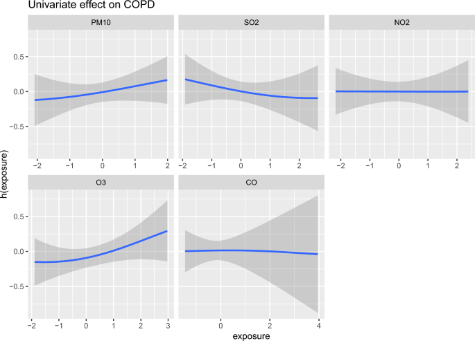
The plots of the univariate effect of \(\text {PM}_{10}, \text {SO}_2, \text {NO}_2, \text {O}_3\), and CO on COPD. The x-axis is the standardized value for each exposure factor, and the y-axis is the corresponding exposure-response function (h) estimate. As the values of \(\text {PM}_{10}\) and \(\text {O}_3\) increase, the probability of contracting COPD increases.
Figure 2 shows the univariate effects of \(\text {PM}_{10}, \text {SO}_2, \text {NO}_2, \text {O}_3\), and CO on COPD. As the standardized value of \(\text {PM}_{10}\) increases, the risk of developing COPD increases linearly. In contrast, as the standardized value of \(\text {O}_3\) increases, the risk of developing COPD exhibits a non-linear upward trend. For \(\text {PM}_{10}\), the estimated effect becomes positive at values greater than approximately 0 (actual average: 49.73 \(\upmu\,\mathrm{g}/\mathrm{m}^3\)). Similarly, for \(\text {O}_3\), the estimated effect becomes positive at values exceeding about 1 (actual average: 0.0470 ppm, corresponding to a standardized value of 1). These findings suggest that the probability of developing COPD becomes higher than the probability of not developing the condition under these circumstances. For \(\text {NO}_2\) and CO, the estimated curves remain flat near 0, indicating no substantial influence in either direction. However, these pollutants may contribute slightly to reduced lung function.
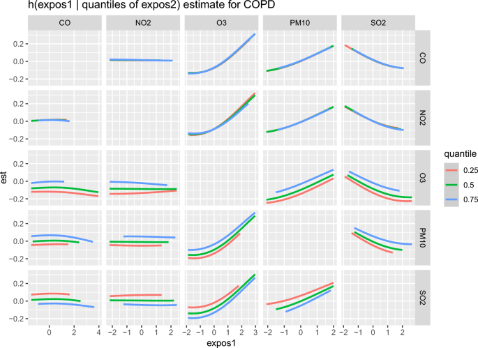
The plots of the joint/interaction effect of \(\text {PM}_{10}, \text {SO}_2, \text {NO}_2, \text {O}_3\), and CO on COPD. The x-axis represents the standardized value for the first exposure factor, and the y-axis represents the exposure-response function estimate for the first exposure factor according to the quantile of the second exposure factor when the values of the remaining exposure factors are fixed.
Figure 3 shows the plots of the joint/interaction effect of \(\text {PM}_{10}, \text {SO}_2\), \(\text {NO}_2\), \(\text {O}_3\), and CO on COPD. When \(\text {SO}_2, \text {NO}_2\), \(\hbox {O}_3\) and CO are fixed at their median, the estimated exposure-response function value increases as the standardized \(\text {PM}_{10}\) value increases as it can seen in the 4th column. Here, when having the same \(\text {PM}_{10}\) value, the exposure-response function value was estimated to be larger as the quantile of \(\text {O}_3\) increased as it can seem in the 3rd row and 4th column. This suggests that when \(\text {PM}_{10}\) and \(\text {O}_3\) are considered together, the potential for developing COPD increases as these values increase.
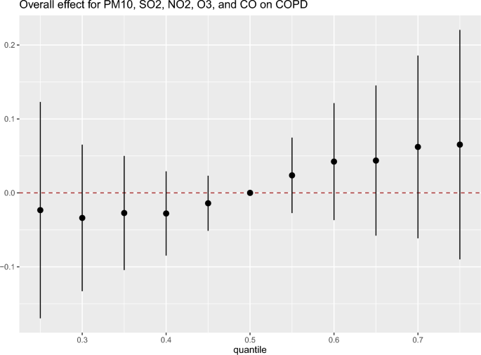
The plots of the overall effect of \(\text {PM}_{10}, \text {SO}_2, \text {NO}_2, \text {O}_3\), and CO on COPD. When all exposure factors are fixed at the 50th percentile (median), these are the relative exposure-factor estimates as they change to the 25th, 30th, \(\ldots\), 70th, and 75th percentiles.
Figure 4 shows the overall effect on COPD for \(\text {PM}_{10}\), including \(\text {SO}_2\), \(\text {NO}_2\), \(\text {O}_3\), and CO. We examined each of the five exposure factors by simultaneously changing them from the 25th percentile to the 75th percentile. As a result, Fig. 4 shows that as the values of exposure factors increase, the potential for developing COPD increases.
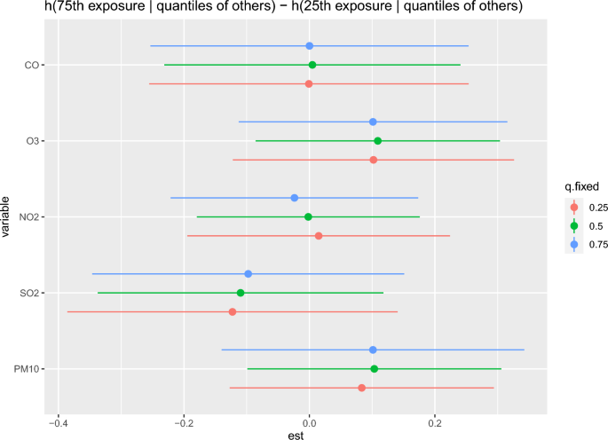
Plot of the single effects of \(\text {PM}_{10}, \text {SO}_2, \text {NO}_2, \text {O}_3\), and CO on COPD. This plot shows the effect of a single exposure to estimate the contribution of each exposure to the total exposure, with all but one of the exposure factors of interest fixed at the 25th, 50th, and 75th quantiles.
Figure 5 shows the single exposure effect to estimate the contribution of each exposure to the total exposure. The y-axis represents a single exposure factor of interest, and the x-axis represents the difference between the exposure-response function estimates at the 75th and 25th quantiles of the single exposure factor of interest, with all but one of the factors of interest fixed at the 25th(red, bottom-line), 50th(green, mid-line), and 75th(blue, top-line) quantiles, respectively. For example, when the remaining exposure factors \(\text {SO}_2, \text {NO}_2, \text {O}_3\), and CO excluding \(\text {PM}_{10}\) are fixed at the 25th, 50th, and 75th percentiles, the difference between 75th percentile and 25th percentile of \(\text {PM}_{10}\) in exposure-response function values is greater than 0. Therefore, it can be said that the potential to develop COPD is greater when \(\text {PM}_{10}\) is at the 75th percentile compared to when \(\text {PM}_{10}\) is at the 25th percentile. Meanwhile, the larger the \(\text {SO}_2, \text {NO}_2, \text {O}_3\), and CO values, the greater the difference in the estimated exposure-response function when the \(\text {PM}_{10}\) value is large, thus it can be interpreted that the potential for developing COPD is greater. In addition, when \(\text {PM}_{10}, \text {SO}_2, \text {NO}_2\) and CO are fixed at the 25th, 50th, and 75th percentile, the potential for developing COPD is greater when \(\text {O}_3\) has a value at the 75th percentile compared to when \(\text {O}_3\) is also at the 25th percentile.
The result of \(\text {PM}_{2.5}, \text {SO}_2, \text {NO}_2, \text {O}_3\), and CO on COPD
Figure S1 shows the plots of the univariate effect of \(\text {PM}_{2.5}, \text {SO}_2, \text {NO}_2, \text {O}_3\), and CO on COPD. As the standardized value of \(\hbox {PM}_{2.5}\) increases, the potential for COPD increases linearly, and as the standardized value of \(\hbox {O}_3\) increases, the potential for COPD tends to increase non-linearly. \(\hbox {PM}_{2.5}\) was estimated to be positive if it had a value greater than about 0, and \(\hbox {O}_{3}\) was estimated to be positive if it had a value greater than about 1, thus the probability of developing COPD can be considered to be greater than the probability of not suffering from COPD. Regarding \(\hbox {NO}_{2}\) and CO, the estimated curves remain straight near 0, thus it can be said that these two air pollutants have affect on reducing lung function.
Figure S2 shows the plots of the joint/interaction effect of \(\text {PM}_{2.5}, \text {SO}_2, \text {NO}_2, \text {O}_3\), and CO on COPD. When \(\hbox {SO}_{2}\), \(\hbox {NO}_{2}\), \(\hbox {O}_{3}\), and CO are fixed at their median, the estimated exposure-response function estimate increases as the standardized \(\hbox {PM}_{2.5}\) value increases as it can seen in the 4th column. Here, when having the same \(\hbox {PM}_{2.5}\) value, the exposure-response function value was estimated to be larger as the quantile of \(\hbox {O}_{3}\) increased as it can seen in the 3rd row and 4th column. This suggests that when \(\hbox {PM}_{2.5}\) and \(\hbox {O}_{3}\) are considered together, the potential for developing COPD increases as these values increase.
Figure S3 shows the overall effect on COPD for \(\hbox {PM}_{2.5}\), including \(\hbox {SO}_{2}\), \(\hbox {NO}_{2}\), \(\hbox {O}_{3}\), and CO. We examined each of the five exposure factors by simultaneously changing them from the 25th percentile to the 75th percentile. As a result, Fig. S3 shows that as the values of exposure factors increase, the potential for developing COPD increases.
Figure S4 shows the single exposure effect to estimate the contribution of each exposure to the total exposure. For example, when the remaining exposure factors \(\hbox {SO}_{2}\), \(\hbox {NO}_{2}\), \(\hbox {O}_{3}\), and CO excluding \(\hbox {PM}_{2.5}\) are fixed at the 25th, 50th, and 75th percentiles, the difference between 75th percentile and 25th percentile of \(\hbox {PM}_{2.5}\) in exposure-response function values is greater than 0. Therefore, it can be said that the potential to develop COPD is greater when \(\hbox {PM}_{2.5}\) is at the 75th percentile compared to when \(\hbox {PM}_{2.5}\) is at the 25th percentile. Meanwhile, the larger the \(\hbox {SO}_{2}\), \(\hbox {NO}_{2}\), \(\hbox {O}_{3}\), and CO values, the greater the difference in the estimated exposure-response function when the \(\hbox {PM}_{2.5}\) value is large, thus it can be interpreted that the potential for developing COPD is greater. In addition, when \(\hbox {PM}_{2.5}\), \(\hbox {SO}_{2}\), \(\hbox {NO}_{2}\), and CO are fixed at the 25th, 50th, and 75th percentile, the potential for developing COPD is greater when \(\hbox {O}_{3}\) has a value at the 75th percentile compared to when \(\hbox {O}_{3}\) is also at the 25th percentile.
The result of \(\text {PM}_{10}, \text {SO}_2, \text {NO}_2\), and \(\text {O}_3\) on \(\hbox {FEV}_1/\)FVC
Figure S5 shows the plots of the univariate effect of \(\hbox {PM}_{10}\), \(\hbox {SO}_{2}\), \(\hbox {NO}_{2}\), and \(\hbox {O}_{3}\) on \(\hbox {FEV}_1/\)FVC. As \(\hbox {PM}_{10}\) became greater than about 1.75 (actual about 75 \(\upmu\,\mathrm{g}/\mathrm{m}^3\)), the exposure-response function was estimated to be negative. Therefore, it can be interpreted that when \(\hbox {PM}_{10}\) becomes greater than about 75 \(\upmu\,\mathrm{g}/\mathrm{m}^3\), \(\hbox {FEV}_1/\)FVC decreases non-linearly. For \(\hbox {NO}_{2}\) (approximately 1.3, actual 0.0462 ppm) and \(\hbox {O}_{3}\) (approximately 2.5, actual 0.075 ppm), if the levels exceed these values, the exposure-response function is estimated to become negative. This suggests that \(\hbox {NO}_{2}\) and \(\hbox {O}_{3}\) contribute to a reduction in the \(\hbox {FEV}_1/\)FVC.
Figure S6 shows the plots of the joint/interaction effect on \(\hbox {FEV}_1/\)FVC for \(\hbox {PM}_{10}\) including \(\hbox {SO}_{2}\), \(\hbox {NO}_{2}\), and \(\hbox {O}_{3}\). In Fig. S6, \(\hbox {PM}_{10}\)-\(\hbox {NO}_{2}\) and \(\hbox {SO}_{2}\)-\(\hbox {O}_{3}\) have an interactive effect with each other. Specifically, when \(\hbox {NO}_{2}\) is at the 25th and 50th percentiles, as the standardized \(\hbox {PM}_{10}\) increases, the exposure-response function estimate becomes smaller, thus \(\hbox {FEV}_1/\)FVC can be seen to decrease. However, when the \(\hbox {NO}_{2}\) level is at the 75th percentile, the exposure-response function estimate for \(\hbox {PM}_{10}\) can be seen to actually increase, and since the three curves intersect, \(\hbox {PM}_{10}\) and \(\hbox {NO}_{2}\) can be seen to have an interaction effect. The relationship between \(\hbox {SO}_{2}\) and \(\hbox {O}_{3}\) can be examined similarly.
Figure S7 shows the overall effect plot on \(\hbox {FEV}_1/\)FVC for \(\hbox {PM}_{10}\) including \(\hbox {SO}_{2}\), \(\hbox {NO}_{2}\), and \(\hbox {O}_{3}\). We examined each of the four exposure factors by simultaneously changing them from the 25th percentile to the 75th percentile. As a result, Fig. S7 shows that as the values of all four exposure factors become larger than the median, the exposure-response function estimate becomes relatively smaller, thus it can be interpreted that \(\hbox {FEV}_1/\)FVC becomes smaller.
Figure S8 illustrates the single-exposure effects, providing an estimate of each exposure’s contribution to the total exposure. In Fig. S8, when other exposures (\(\hbox {SO}_{2}\), \(\hbox {NO}_{2}\), \(\hbox {O}_{3}\)) within \(\hbox {PM}_{10}\) are at the 25th and 50th percentiles, the difference in the exposure-response function estimates between the 75th and 25th percentiles of \(\hbox {PM}_{10}\) is negative. This indicates that the exposure-response function estimate for the 75th percentile of \(\hbox {PM}_{10}\) is smaller than that for the 25th percentile. Furthermore, when \(\hbox {SO}_{2}\) is at the 25th and 50th percentiles, \(\hbox {NO}_{2}\) is at the 25th, 50th, and 75th percentiles, and \(\hbox {O}_{3}\) is at the 75th percentile, with all other exposure factors fixed at the median, a change in the value of the exposure factor from the 25th to the 75th percentile can be observed. This suggests that the \(\hbox {FEV}_1/\)FVC decreases as these exposure levels increase.
The result of \(\text {PM}_{2.5}, \text {SO}_2, \text {NO}_2\), and \(\text {O}_3\) on \(\hbox {FEV}_1/\)FVC
Figure S9 shows the plots of the univariate effect of \(\hbox {PM}_{2.5}\), \(\hbox {SO}_{2}\), \(\hbox {NO}_{2}\), and \(\hbox {O}_{3}\) on \(\hbox {FEV}_1/\)FVC. In Fig. S9, unlike Fig. S5, the exposure-response function for \(\hbox {PM}_{2.5}\) was estimated to be almost 0. Nonetheless, when the \(\hbox {PM}_{2.5}\) standardized value is greater than about 3, the exposure-response function estimate is estimated to be negative, indicating a decrease in \(\hbox {FEV}_1/\)FVC. Likewise, \(\hbox {NO}_2\) and \(\hbox {O}_3\) can be interpreted to reduce \(\hbox {FEV}_1/\)FVC if they are above a certain value.
Figure S10 shows the plots of the joint/interaction effect on \(\hbox {FEV}_1/\)FVC for \(\hbox {PM}_{2.5}\) including \(\hbox {SO}_{2}\), \(\hbox {NO}_{2}\) and \(\hbox {O}_{3}\). In Fig. S10, \(\hbox {SO}_{2}\)-\(\hbox {O}_{3}\) have an strongly interactive effect with each other.
Figure S11 shows the overall effect plot on \(\hbox {FEV}_1/\)FVC for \(\hbox {PM}_{2.5}\) including \(\hbox {SO}_{2}\), \(\hbox {NO}_{2}\) and \(\hbox {O}_{3}\). We examined each of the four exposure factors by simultaneously changing them from the 25th percentile to the 75th percentile. As a result, Fig. S11 shows that as the values of all four exposure factors become larger than the median, the exposure-response function estimate becomes relatively smaller, thus it can be interpreted that \(\hbox {FEV}_1/\)FVC becomes smaller.
Figure S12 illustrates the single-exposure effects, providing an estimate of each exposure’s contribution to the total exposure. In Fig. S12, when other exposures (\(\hbox {SO}_2\), \(\hbox {NO}_2\), \(\hbox {O}_3\)) within \(\hbox {PM}_{2.5}\) are at the 50th and 75th percentiles, the difference in the exposure-response function estimates between the 75th and 25th percentiles of \(\hbox {PM}_{2.5}\) is negative. This indicates that the exposure-response function estimate for the 75th percentile of \(\hbox {PM}_{2.5}\) is smaller than that for the 25th percentile. Furthermore, when \(\hbox {SO}_{2}\) is at the 50th and 75th percentiles, \(\hbox {NO}_{2}\) is at the 50th and 75th percentiles, and \(\hbox {O}_{3}\) is at the 75th percentile, with all other exposure factors fixed at the median, a change in the value of the exposure factor from the 25th to the 75th percentile can be observed. This suggests that the \(\hbox {FEV}_1/\)FVC decreases as these exposure levels increase.