A significant difference was seen in the impacts of genotype, environments, and genotype by environment interaction (GEI) (p 1). These findings showed that fresh cowpea yield (t/ha) was influenced by the ten cowpea genotypes and the nine environmental conditions (three locations and three growth seasons) under study. These findings agree with those of Kindie et al. (2021)21, Kusi et al. (2025)22, and Tariku et al. (2018)23, who evaluated 25, 23, and 16 cowpea genotypes in six, four, and seven environments, respectively. These findings imply both the appropriate and desired genetic diversity among the many studied genotypes, in addition to the variation between locations and growing seasons under investigation.
With a value of 86.15%, the environment’s sum of squares had the highest component of all the sums of squares. According to the findings, the environment is the primary source of variation since it contributed significantly to the sum of squares for fresh cowpea production, accounting for the main effect. Atakora et al. (2023)24, who obtained comparable observations and connected them to the environment and their interaction, bolster this claim. The genotypes and GEI under investigation came in second and third, with values of 6.54% and 4.54%, respectively. Opposite, it was confirmed that GEI was highly significant and had a noteworthy effect on genotypic performance in various contexts since its sum of squares was higher than the genotypes25. This suggests that the fresh cowpea yield (t/ha) varied over time due to significant heterogeneity in the genotypes’ responses. The best genotypes under the studied sites in the growing seasons can be chosen with the help of these differences. Genotype, environment, and GEI all had a substantial impact on cowpea dry matter yield26. The GEI component’s sum of squares yielded eight principal component axes (PCs). For the first five principal components (PC1–PC5), the mean squares were significant (p 24,27,28,29. This outcome is consistent with the recommendation made by Gauch et al. (1996)30 that the AMMI model be used to estimate the most accurate model utilizing the first two PCs.
According to Eisemann et al. (1990)31, considerable GEI should be utilized rather than disregarded. Exploiting GEI entails analyzing and interpreting genotypic and environmental variations to determine the stability of performance of various genotypes over a range of contexts. As a result, stability could be calculated and the type and extent of GEI could be investigated, something that a typical analysis of variance cannot do32. While the GE interaction suggested that some genotypes were uniquely adapted to particular environments, the observation of significant main effects of genotypes and environments demonstrated that some genotypes were stable across settings. As a result, selection efficiency and, to a greater extent, variety recommendations for production are impacted by this variation in performance between settings. The GEI impacts can be lessened by choosing stable genotypes in a variety of settings4.
Mean performance
The fresh cowpea yield (t/ha) data in Table 2 revealed a substantial variety (p 25. Our results showed that Sids location increased the fresh cowpea yield (t/ha) of all genotypes examined in all growing seasons, followed by Sakha and Ismailia locations. Compared with the growing seasons, the fresh cowpea yield (t/ha) of most genotypes studied increased in the 2023 growing season at the Ismailia and Sakha locations and in the 2021 growing season at the Sids location. According to these results, certain genotypes showed good behavior, as evidenced by their high ability to generate fresh cowpea yield (t/ha) in various environments, while other genotypes experienced more negative consequences. Due to the positive interaction between the temperature and humidity, which can interact in complex ways, with temperature affecting the rate of water loss and humidity affecting the availability of water for plants. Understanding these relationships is crucial for developing effective forage management strategies, such as choosing appropriate plant species. The grand mean fresh cowpea yield (t/ha) was significantly higher at the Sids location than at the Ismailia and Sakha locations, with values of 30.46% and 4.94%, respectively, throughout all genotypes and all growing seasons. The studied locations differed in seasonal temperatures and relative humidity. The growing seasons during which the experiments were carried out also differed in terms of meteorological data. High temperatures and low relative humidity were noted in the Sids region, followed by the Ismailia region and the Sakha region, according to meteorological data. Seasonal temperature and relative humidity levels influenced the performance of certain genotypes, which only flourish in favorable conditions; as a result, even minor deviations from the prevailing climatic conditions can hurt growth and yield24. At the Sids location, the G5 and G3 genotypes in the 2021 and 2022 growing seasons produced a maximum fresh cowpea yield with values of 86.59 and 82.88 t/ha, respectively. While G10 had the minimum fresh cowpea yield (t/ha) at all locations in all growing seasons, and the lowest value was observed at the Ismailia location in the 2021 growing season. This may be due to Ismailia location differing in factors like temperature, rainfall, soil type, and sunlight, which can significantly impact a genotype’s growth, development, and yield. Also, a genotype might perform exceptionally well in one location but poorly in another, highlighting the presence of genotype-by-environment interaction. Thillainathan and Fernandez (2002)33 state that consistent outcomes in a variety of environments (locations and/or years) may lead to yield stability. The crossover kind of GEI influence was shown by the different yield ranking of genotypes in different environments34. The GEI effect was identified as a crossover type (changes in a genotype’s rank from one environment to another) by the inconsistent yield ranking of genotypes from environment to environment (Crossa 1990)35. According to the study’s findings, the genotypes that were evaluated may not be able to adapt to all of the environments that were examined4,36,37.
GxE heatmap analysis
As seen in Fig. 1, a visual comparison of the impacts of growing seasons and locations on the genotypes was produced using GxE heatmap analysis of fresh cowpea yield (t/ha). Two dendrograms were identified by the G x E heatmap analysis: the nine environments on top and those that affected the distribution of the ten cowpea genotypes on the left. The environments were divided into two distinct groups using the top dendrogram. E1, E2 and E3 environments made up the group (A) The other environments are included in the group (B) Ten genotypes could be categorized into groups (C and D) based on the left dendrogram. There was only one genotype (G3) in Group (C) Group D was split up into five different clusters. Whereas the genotypes between clusters differ and have the greatest genetic distance, the genotypes within clusters have the least variance and genetic distance. Each of the first and third clusters consisted of one genotype (G10 and G1, respectively). While each of the second and fourth clusters were composed of two genotypes i.e., G3 and G5, as well as G2 and G7, respectively. The fifth cluster consisted of the remaining genotypes (G4, G6, G8 and G9). The G3 genotype gave the highest fresh cowpea yield (t/ha) in the E1, E2, E3, E5, and E8 environments compared with the other studied genotypes in these environments. Also, the genotypes G5 in the E4 environment, G8 in the E6 environment, and G2 in the E9 and E7 environments had the best fresh cowpea yield (t/ha). On the other hand, the genotype G10 had the lowest fresh cowpea yield (t/ha) in all environments under study. Generally, GxE heatmap analysis of fresh cowpea yield (t/ha) classified the genotypes and environments into different separate clusters, and the genotypes G3, G5, G2, and G8 had the best fresh cowpea yield (t/ha) across most environments under study. The findings of the GxE heatmap showed significant variations in fodder yields between genotypes38. This suggests that the performance of the genotypes varied among the test conditions. It is possible to speculate that variations in abiotic elements like soil, vegetation, and rainfall could be the cause of the variations in genotype potentials between test environments; climate variations between years could also play a role22.
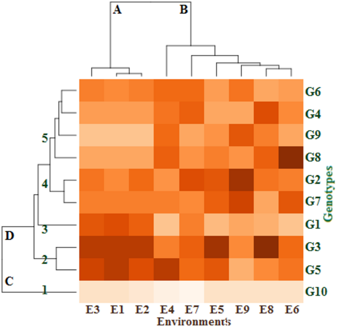
Dendrogram of classified ten genotypes in nine environments by cluster analysis. The color of each block deepens with the increase of the corresponding fresh cowpea yield, then the color depth decreases, and the color scale ranges from mild for the moderate fresh yield to white for the lowest fresh yield. The environments and genotypes key names can be found in Tables 2 and 5, respectively.
Multivariate stability parameters
To maximize the benefits of GEI and enhance the accuracy and refinement of genotype selection, yield and performance stability should be taken into account simultaneously39. Accordingly, stability statistics can be used as a compromise technique to identify genotypes that are suited to challenging growing conditions and to choose genotypes with a moderate yield and good stability according to El-Hashash and Agwa (2018)40. Using a variety of multivariate stability parameters, stability assessments of fresh yield (t/ha) for ten cowpea genotypes under nine environmental variables (three sites in three growing years) were carried out, as shown in Table 3. The G3 genotype gave the highest mean response for fresh cowpea yield with values of 63.55 (t/ha), followed by G5 (62.11 t/ha), G2 (60.87 t/ha), G7 (59.80 t/ha), and G8 (59.31 t/ha) in the nine different environments. The eight genotypes performed better than the grand mean (58.32 t/ha) when the mean response was used as the first criterion for assessing the genotypes under the studied environments. Generally, the previous genotypes recorded the highest values and indicated the most stable genotypes based on the Yi statistic. While, with fresh cowpea yield values of 47.84 (t/ha) and 56.69 (t/ha), the G10 and G9 genotypes showed the lowest mean response, respectively.
The genotypes would be more stable across settings, according to the minimal values of the following statistics: ASTAB, ASI, ASV, AVAMGE, Da, Dz, EV, FA, MASI, MASV, SIPC, Za, and WAAS. The genotype G7 showed a good balance between stability and yield, and it showed above-moderate performance in fresh cowpea yield performance, with the lowest values of all the evaluated multivariate stability parameters. Additionally, the genotypes G3, G5, G8, and G2 demonstrated stability, exhibiting high and moderate fresh cowpea production performance. In contrast, the genotypes G1, G9, and G10 (low yield) showed the greatest multivariate stability parameter values, indicating that they are unstable. According to Pour-Aboughadareh et al. (2022)41, only a small number of AMMI model factors, such as MASV, assisted in identifying stable high-yielding genotypes, even though the bulk of them contain a dynamic concept of stability. Using AMMI-based stability metrics, Goa et al. (2022)25 reported similar results in cowpea, John et al. (2025)42 in rice and Mengistu and Abu (2023)43 in sunflower. They concluded that the majority of AMMI statistics are appropriate for identifying stable genotypes. According to Mbeyagala et al. (2021)44, our findings thus validate the applicability of ASV in identifying stable and high-yielding cowpea genotypes. ASV is advised for GxE analysis and cultivar identification in cereals and legumes due to its predictive value45.
The multivariate stability parameters were used to rank ten genotypes. The results showed that the ranks of genotypes for ASI and ASV parameters, Da and FA parameters, Dz and EV parameters, and Za and WAAS parameters were identical in fresh cowpea yield (Table 3). As a result, it is sufficient to use one of these parameters. Because of this, it might be regarded as a suitable substitute for one another. Additionally, the majority of the multivariate stability parameters under investigation showed frequently comparable ranks for the genotypes, indicating that these parameters are equal for genotype selection. They might therefore be regarded as suitable substitutes for one another. All of the stability measures nearly showed a similar tendency in identifying stable genotypes, according to studies by Anuradha et al. (2022)46 in finger millet and Cheloei et al. (2020)47 in rice that used the same set of stability indices.
Rank correlation among mean yield and multivariate stability parameters
The Spearman’s rank correlation coefficients, which were calculated for each pair of multivariate stability parameters for ten genotypes under nine environments, are shown in Table 4. rASI, and rASV parameters, rDa and rFA parameters, rDz and rEV parameters, and rZa and rWAAS parameters were found to have a highly significant and perfect rank correlation coefficient (r = 1.00). According to these findings, the genotype ranks by these stability metrics were the same, as Table 5 illustrates. Mean response showed significant and positive correlations with rASI, rASV, rAVAMGE, rMASI, rMASV (0.05), rZa, and rWAAS (0.01), and these measurements can be utilized to choose high fresh yield and stable genotypes. Also, positive rank correlation coefficients for rYi with the other multivariate stability parameters under investigation were noted. The non-significant relationship between mean yield and stability factors suggests that stability parameters provide information that average yield cannot48.
Significant rank correlation coefficients (P 46, John et al. (2025)42 and Mengistu and Abu (2023)43 that all of the AMMI-based stability parameters showed a positive and significant association with one another. The strong association between these stability statistics is indicated by their significant positive correlation, which also implies that these parameters would have comparable functions in the effective stability ranking of genotypes and vice versa. As a result, these stability models imply that they offer similar information about genotype rankings for stability across different settings. Additionally, stable and high-yielding genotypes can be selected using any one of these factors, or any combination of them. It is not appropriate to interpret these characteristics as distinct processes49.
AMMI biplot
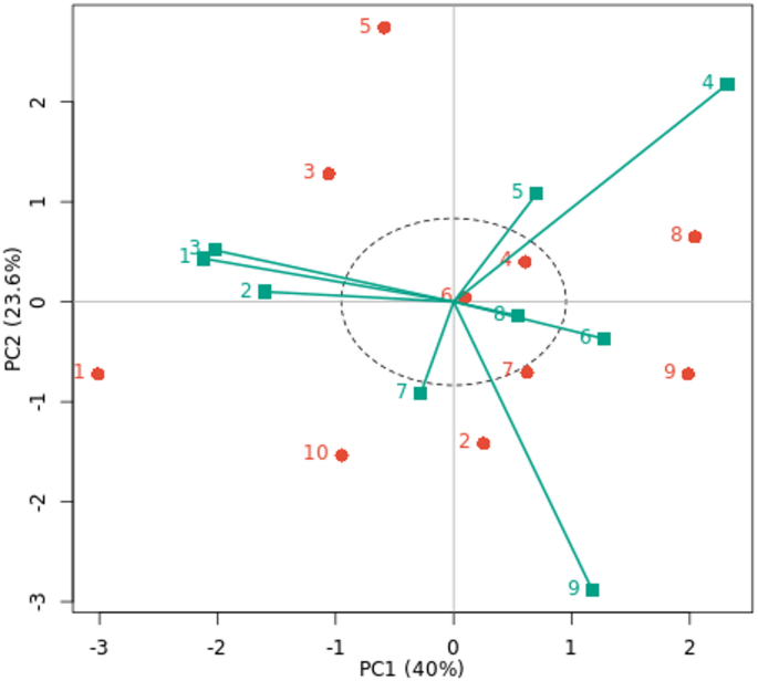
The AMMI biplot was used to analyze fresh yield (t/ha) for ten cowpea genotypes across nine environments, as seen in Fig. 2. Of the ten genotypes under nine environments, PC1 and PC2 explained 40.0% and 23.6% of the total variance, respectively, accounting for the first two PCs’ 63.6% contribution to the entire variability in the data. This suggests that the first two PCs of genotypes and environments predicted the interaction of ten cowpea genotypes with nine environments. Therefore, the best-performing genotypes across nine environments can be found using PC1 and PC2. This is consistent with the advice of Abiriga et al. (2020)29 and Zobel et al. (1988)50, who suggested that the first two PCs could predict the most accurate model for AMMI. According to Kusi et al. (2025)22, the interaction’s PC1 and PC2 accounted for 51.35% and 32.23% of the GEI sum of squares, respectively. In a study by Tunc et al. (2025)51, 84% of the variation was explained by PC1 and PC2. This demonstrated that the AMMI model well captured how genotypes performed when exposed to environmental influences. Also, according to Gauch et al. (2008)17, cross-validation of the yield variation explained by GEI is possible using the AMMI model with the first and second multiplicative terms. The most stable genotypes that contributed less to GEI were those that were collected and placed near the biplot origin. The genotypes G7, G6, and G4 are stable in all studied environments because they are near the biplot origin with reduced GEI. However, genotypes G10 and G1 are unstable because they are further distant from the origin and contribute more to GEI in all studied environments. The AMMI stability values offer further insight into genotype variation, while the AMMI biplot shows the link between genotypes and environments27. Characterizing GEI across cowpea genotypes and identifying genotypes with a favorable balance of stability and improved yield performance were made possible by the application of AMMI44.
There is a positive correlation between environment and genotype when they are positioned close to one another in the biplot, suggesting specific adaptation52. For example, specific adaptation was demonstrated by the G3 and G5 genotypes with E1, E2, and E5 environments and the G7 and G2 genotypes with the E9 environment. The E4 and E9 environments showed the longest vectors and the highest fresh cowpea yield (t/ha). This implies that the GEI determination is significantly influenced by these environments. Short vectors were seen closer to zero and closer to the biplot origin for the E1, E2, and E3 environments. Additionally, there is less than a 90-degree angle between the E5, E4, and E6 environments and the E7 and E9 environments. Because of this, these environments are less dynamic and more stable, which virtually guarantees that all genotypes will perform better there. These genotypes’ optimal adaptability to their different habitats is demonstrated by the AMMI model’s selection of them in those environments22. These results are in line with those for cowpea reported by Ghazy. Mona et al. (2017)53, Kindie et al. (2021)21 and Kusi et al. (2025)22. They saw cowpea genotypes that were wanted in both favorable and unfavorable conditions, as well as genotypes that were solely wanted in either a favorable or unfavorable setting.
GGE biplot analysis
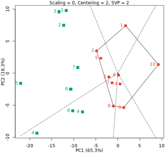
The GGE biplot was created by plotting the PC1 and PC2, which were produced by applying singular value decomposition to environment-centered yield data14. The average environment coordination (AE) technique, which is based on genotype-focused singular value partitioning (SVP), was utilized to assess genotype yield stability using average PCAs in all environments. The GGE biplot is a simple technique for assessing the influence of genotype on the environment in cowpea and offers useful information about the genotypes and environments under study54. Both the first two PCs GGE biplots explained 65.3% and 16.3% (81.6%) of the total G + GE variation across the nine environments under study, respectively. According to Kusi et al. (2025)22 and Owusu et al. (2020)55, the first two principal components accounted for 79.54% and 69.59% of the total yield variance of cowpea throughout the studied settings, respectively, according to the GGE biplot results. Additionally, based on the results by Kusi et al. (2025)22, PC1 and PC2 explained 53.68% and 25.86%, respectively. According to Horn et al. (2018)27 and Matova and Gasurae (2018)56, the GEI can be well explained by the first two major components. In Fig. 3, G1, G3, G8, G9 and G10 genotypes formed the polygon vertices in nine environments under study. These genotypes are dispersed in all directions from the biplot origin, and the polygon encompasses all other genotypes. With the GGE biplot polygon of “which-won-where”, the environments were divided into two sectors, with the top of each sector (vertex) containing the best fresh cowpea yield in the environments located within each sector. Our results were consistent with Yan et al. (2007)57, who state that the division of settings into discrete sectors suggests that each sector has its high-yielding genotypes. This implies that the test environments might be combined to form mega-environments, which are larger entities. Using a GGE biplot, the cowpea genotypes were separated into four and three mega-environments, respectively21,26. Therefore, the best fresh cowpea yield was obtained by genotype G8 in the E4, E6, and E9 environments and genotype G3 in the other environments. The genotypes inside the polygon are less ecologically fit than those at the vertices. The relations between the different genotypes and the environment was graphically represented by the GGE biplot of the “what won where” analysis. In terms of superior genotypes in connection with surroundings, this observation is consistent with that of Horn et al. (2018)27 and Atakora et al. (2023)24.
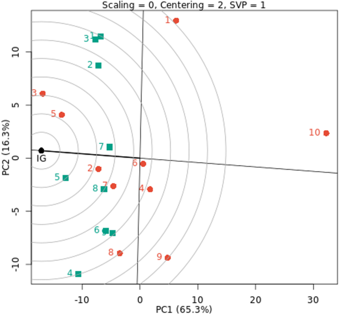
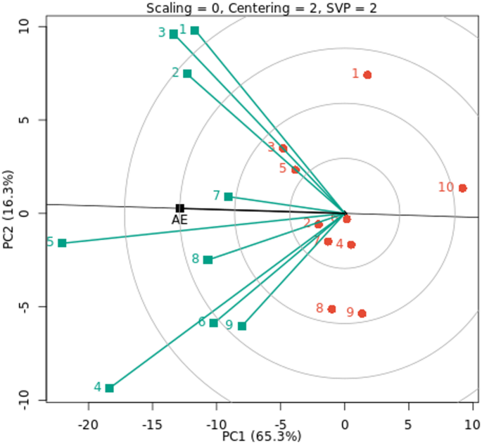
The GGE biplot of the decorativeness vs. representativeness view is a useful tool for evaluating test environments and can be used to identify a basic set of representatives and discriminating test environments (Fig. 4). Finding test environments, precisely defining genotype differences, and providing the data required for plant breeders to make an election are all critical. Our findings showed that the test environments E4 and E5 are more representative of other test environments because they have the longest vector and the lowest angles with AE, followed by the environments E1, E2, and E3, as according to Yan et al. (2007)57. These findings imply that these environments are optimal and possess the greatest ability to differentiate across genotypes, promoting the selection of superior genotypes for fresh cowpea yield. Additionally, in test environment E7, a tiny angle with AE and a medium vector was discovered. Yan and Rajcan (2002)58 state that the most desired genotype is the one that is closest to the graph of the ideal environment. Thus, G7 and G2 are the most stable and productive genotypes in the nine environments under study, as well as genotypes G3 and G5, which are located close to E1, E2, and E3 environments. Strong positive correlations were observed for E7 with E2 and E3, among E1, E2, and E3 environments, and between E5 and E6 environments because the angles between them are acute. E9 with the E1, E2, and E3 environments had a slight positive correlation. While moderate positive correlations were found between the other environments. The cosine of the two environments’ angles and their length vectors indicates how similar (covariant) they are19. As a result, the ray lines divided the environments into two groups: the first group included the E1, E2, E3, and E7 environments, while the second group included the other environments under study. According to Yan and Kang (2002)59, the optimal genotype is determined by two factors: (i) it has the maximum yield of the complete dataset, and (ii) it is stable because it is found on the AEC abscissa. Nonetheless, the environment is always the primary source of diversity, and plant breeding must give it top priority60.
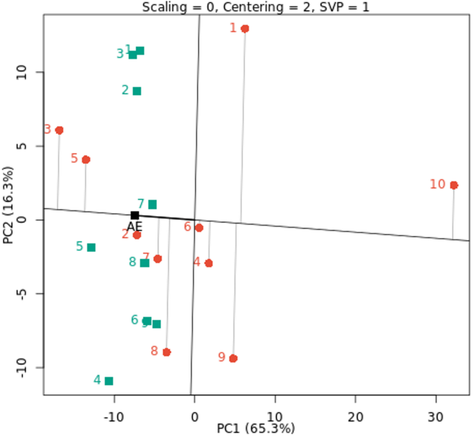
The representation of genotypes that combine high mean performance and stability is one notable feature of the GGE biplot graph. The genotypes are categorized according to their average fresh cowpea yield, as shown by the arrow sign on the AE (Fig. 5). G6, G4, G1, G9 and G10 genotypes had below-average means, whereas other genotypes had above-average means. Therefore, the lowest fresh cowpea yield was recorded by G10, G9, and G1 genotypes under all nine environments, and are more changeable and unstable. On the other hand, the other studied genotypes were registered as moderate to high for fresh cowpea yield across all nine environments under evaluation. G2 and G7 were the most stable genotypes; they were located almost on the AE abscissa and had a near-zero projection onto the AE ordinate. Compared to the other genotypes, the stable G8, G5, and G3 genotypes yield fresh cowpeas with a moderate to high mean yield. Despite being an effective tool for comprehending GEI, GGE biplot analysis has many drawbacks. This approach disregards environmental impacts even if it is useful for visualizing genotype performance and selecting optimal genotypes and environments51.
In all environments examined, the genotypes with above-average mean performance were ranked as G3, G5, G2, G7, and G8, as illustrated in Fig. 6. These genotypes are more stable and have higher mean cowpea yields than the others. However, other genotypes, including rank G10, G9, G1, G4 and G6, were unstable and performed below average on average across all situations. Similar findings about the graphical representation of biplots of some genotypes’ performance by comparing various settings have been reported by Horn et al. (2018)27 and Atakora et al. (2023)24.
Across nine environmental circumstances, the most stable genotypes were G3 by mean response, G7 and G2 by AMMI-based stability parameters, and AMMI and GGE biplot analysis. Because of its capacity to fix atmospheric nitrogen and generate robust roots, the legume family is generally regarded as one of those that can withstand climate change. Regarding G7 and G2, they possess a few key traits that could enable them to adapt to climate change:
1.
Hair is present on the leaf’s surface. This makes it more disease-resistant.
2.
The thickness of the leaf is considered more than that of other lines.
3.
They have the greatest number of branches.
4.
The leaf color is darker green than other strains. This indicates that the process of photosynthesis is carried out with higher efficiency.
5.
There is a thin, waxy layer on them, which helps prevent quick water loss and is tolerant of drought stress.